2D NMR Processing Tour


2D NMR Processing Tour |
|
|
(Not available in Mnova Lite)
1D experiments contain a wealth of information but this information is often obscured due to signal overlap. Homonuclear couplings are often more readily and rapidly determined by extension into a second dimension. Heteronuclear couplings (1H-13C for example) are much easier to determine using two frequency dimensions. 2D experiments which use one frequency dimension and some other variable on the other axis (the DOSY processed STE experiment for example with diffusion coefficient on one axis) exist but this tour will concern two frequency (chemical shift) dimensions.
These 2D spectra are collected as time domain data dependant upon two time variables (t1 and t2) and after two orthogonal Fourier transformations a frequency spectrum which is a function of two frequency variables results. The general scheme for these two dimensional experiments is shown in the pulse sequence below:
In the Preparation Time, the sample is excited by one or more pulses and the spin system is placed in a non-equilibrium state which will evolve later. During the evolution period, the resulting magnetization evolves freely. Each signal will evolve with its characteristic frequency. Then follows the Mixing Time containing a further pulse or pulses; it is in this period that, for example, magnetization, may be transferred from proton to 13C during indirect detection. Finally the signal is recorded (detected) as a function of the second time variable, t2; the signal has, however, been frequency-labelled as a function of t1. After acquiring a bidimensional experiment, you will have a matrix of data; the rows contain data collected at fixed values of t1 with t2 varying; they are, in fact, normal 1D data FIDs. The columns contain data collected at fixed values of t2 with t1 varying and are "synthetic" 1D FIDs. This matrix will be fourier transformed twice, once for the rows and again for the columns. In this way, the time dimensions (t1 and t2) are converted into frequency dimensions (f1 and f2). In a 2D-NMR experiment we can find any nucleus represented on either of the dimensions of the spectrum, so the spectrum can show correlations between the same nuclei (1H/1H) or different nuclei (such as 1H/13C, 1H/15N, 1H/31P, etc...). In a 2D-NMR spectrum, the acquisition dimension (t2) is the dimension in which we can obtain the greater number of data points without a considerable increase of the acquisition time. On the other hand, each point acquired in dimension t1, multiplies the necessary number of scans, considerably increasing the total acquisition time. For this reason, in many cases the number of data points acquired along the t1 dimension is much smaller than along t2, although this number of points must always be must always be sufficient to provide adequate f1 resolution. The "synthetic" f1 FIDs are generally truncated and may benefit from forward linear prediction. Processing of 2D NMR data sets with Mnova is almost as easy as processing 1D NMR data. You simply select the FID file (or SER file in Bruker) and the 2D spectrum appears on your screen without the need to touch a single button.
In this tutorial we will show how to process a 2D experiment. This tour will guide you through all the necessary steps to process, display, and print out two dimensional spectra with Mnova. Before you attempt to process a 2D spectrum, please read the 1D NMR Processing Tour since you need to be able to process 1D spectra also.
Multidimensional (or bidimensional) data processing requires only a few new concepts when compared with 1D NMR data processing. A 1D-NMR spectrum can be considered as a single vector of data points and its transformation into the frequency domain only requires only one FT. In the case of 2D spectra we have a two dimensional matrix of points and it is necessary to Fourier transform both rows and columns.
In 2D homo- and heteronuclear NMR the matrix of points results from an array of 1D FIDs which are functions of t2 due to their detection (sampling of the FID at intervals of delta-t2) and t1 since each successive FID the value of t1 which determined the evolution time, is incremented. The first row has t1=0, the second row has t1=Δ1, the third row has t1=2Δ1 and so on. The same happens with the data columns, although in this case the sample interval is different (Δ2).
As you can see in the picture above, the first step is the application of the FT along the rows of the matrix; to obtain a new matrix (interferogram) where each row corresponds to an increasing value of t1 and each column to a running frequency variable ω2. Next the columns are subjected to a FT to obtain the final matrix (2D spectrum) where the frequency axes (ω1) corresponds to the evolution in t1, while ω2 corresponds to the evolution in t2.
This 2D data can be processed using apodization functions and once you obtain the 2D spectrum, you can apply a phase or a baseline correction as with 1D processing. One important point is that processing operations need to be performed along each dimension. In Mnova, the processing is always started along the acquisition dimension, and finished along the indirect dimension.
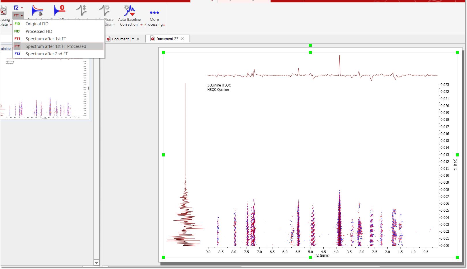
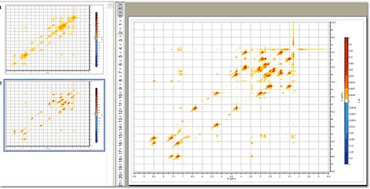
In this example we will use a Bruker spectrum so you will need to select the ser file. Once you do so, you will immediately obtain the processed spectrum:
The program has performed the following set of operations on the fly:
1.Automatic file format recognition: The program identifies this file as a Bruker file and uses the corresponding filter to decipher the data 2.For each dimension:
The user can break the processing after the first FT along the direct dimension and also before the second FT (in t1)
Baseline Correction
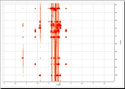
From the figure above, baseline artifacts along the indirect (f1) dimension are apparent. They can be easily removed by the baseline correction procedure. Select this option by clicking on the 'Baseline Correction' icon
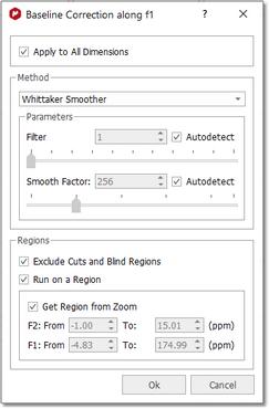
Baseline correction will be applied to the currently active dimension unless the 'Apply to All Dimensions' option is checked.
You can exclude cuts and blind regions or select a region of interest to apply the baseline correction.
In our present situation, as the current processing dimension is f2, baseline correction will take place only along this dimension. This is not appropriate for our case as it is evident that baseline distortions are present mainly along the indirect (f1) dimension. We can simply set the processing dimension to f1, but it is even simpler to check the 'apply to all dimensions' option in the baseline correction dialog box. After applying the correction using default values, this is the resulting spectrum:
The user can show the traces of the 2D-NMR spectrum, just by clicking on 'Show Traces' icon
See also 'Show traces in 2D-NMR'
More on real time frequency domain processing
In the 1D NMR Processing section, we described the real-time frequency domain processing concept. Diagonal Suppression of homonuclear 2D experiments represents another example of this concept. This technique is typically carried out in the mixed time-frequency domain (interferogram). However, this is something you do not need to know in Mnova. You can suppress the diagonal while the transformed spectrum is on the screen.
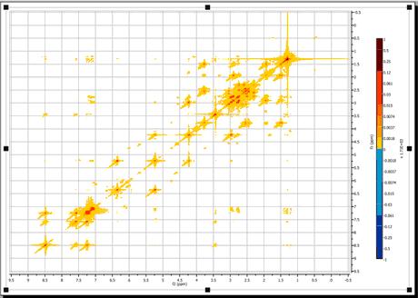
For example, the figure below shows a 2D magnitude spectrum:
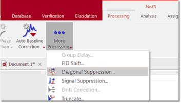
To suppress the diagonal, just click on the small arrow at the right-hand side of the FT toolbar button (see below) and select the Diagonal Suppression command:
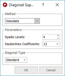
Mnova provides different algorithms for this task. In this example we will select the Wavelet method
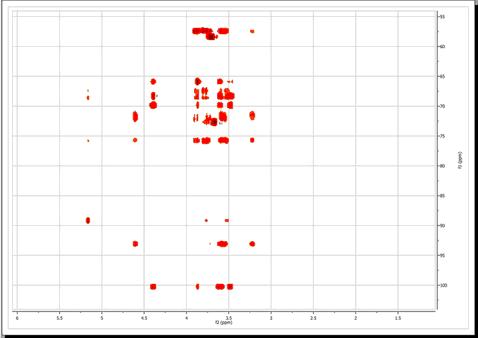
And this is the resulting diagonal-free spectrum.
Note that in the figure above there are two pages, the first one containing the 2D spectrum with its original diagonal, and the second one after the diagonal has been removed.
See also |