Fourier Transform

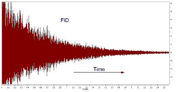
Basic concepts on FT

Modern NMR involves pulse RF energy to excite all frequencies at once. Immediately after the pulse, the signal is detected as a time domain interferogram which contains  the sum of all the damped-sinusoid signals emitted by the sample at the various nuclear resonance frequencies.

The signal will decay with time as various relaxation mechanisms either dephase the magnetization in the X-Y plane or return the magnetization to the Z axis. The resulting   interferogram is called the free induction decay (FID, see figure below)

If you pay close attention to the FID shown in the figure above you can appreciate that it is composed of several frequencies. Moreover, if you were able to count the number of peaks and valleys in a given period of time (e.g. 1 second), you might be able to measure the periods and calculate the frequencies of some of the signals composing the FID.

In ‘real’ life, you don’t need to do this conversion by hand. Fortunately, Jean-Baptiste Joseph Fourier suggested, while working a study of heat flow, that any function of a variable, can be represented by a sum of multiples of sinusoidal harmonics of that variable. This work was later developed into the Fourier Series.

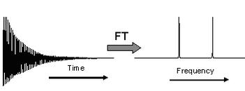
Fourier's proposals led, in part, to the development of a linear mapping operator which maps a given function to other functions and in our particular case, functions of time to functions of frequency.  The operator was named the Fourier Transform in Fourier's honour. In short (math details are beyond the scope of these documents), the Fourier Transform or FT is the mathematical process that converts the time domain function (the FID) into a frequency domain function (the spectrum) as illustrated below:

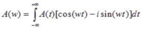
Thus, FT is a mathematical procedure which generates the spectrum from the FID. It searches through the FID for frequency information and allows a plot of signal intensity versus frequency to be generated. When the frequency information is well defined, the peaks will be sharp, but if the information is not precise, the peaks will be broader.

The Continuous Fourier Transform nitty-gritty involves the equation:

where A(w) is the intensity of the signal as a function of frequency, A(t) is signal intensity of the FID as a function of time and i is (-1)1/2.

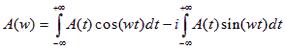
Separating the real from the imaginary part, we have:

The real part can be taken as the signal component which starts off in phase with the receiver reference oscillator, while the imaginary part is that which starts off 90 degrees out of phase with the receiver reference.

The original Fourier Transform is defined for functions of a continuous variable:  To meet the needs of pulse NMR where the FID is sampled at short but discreet intervals, the so called Discrete Fourier Transform (DFT) is used. When the signal strength has been measured with discrete time-interval sampling, the Fourier integral is replaced by:

where N is the number of samples, n is the nth sample and 2πk is a multiplier which converts point n, into the value corresponding to wt (in rad/s). If we have a collection (named A) of N signal points as a function of time,  the calculation of the applicable arrays of real and imaginary frequency points is quite straightforward and can be easily carried out with a computer.  

The calculations with many points are obviously slow (though with current computers, they are extremely fast), but the more points, the smoother the plots will be. In order to reduce the computation time we can use the Cooley-Tukey fast-Fourier algorithm (FFT), reducing the number of calculations from N*N for the DFT to Nlog2N for the FFT.  If N is 1024 samples the reduction is from 1048576 to 7098, a 93% time reduction.  This algorithm has the special restriction that N must be a power of 2. (In cases where the number of points is not a power of 2, Mnova will extend the size of the FID by adding zeros to the next higher power of 2).

The Cooley-Tukey algorithm for the FFT achieves this stunning reduction in computation time in part by a process called "bit reversal" which avoids repetitions of internal vector component calculations. The algorithm also saves time by recognizing the orthogonality of certain calculations, allowing the one vector to be calculated from another just by changing an algebraic sign, or reversing sine and cosine terms. This process is an example of the general technique of divide and conquer algorithms apparent in many traditional implementations, in which the FT is divided in other more and more small FTs.

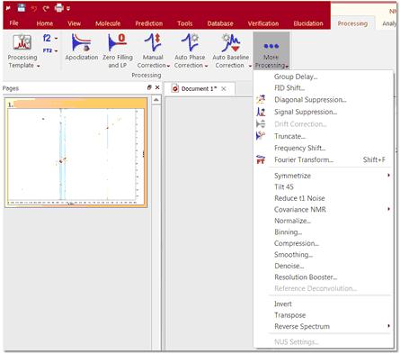
Although, as explained in the items dedicated to 1D and 2D NMR Processing, all processing parameters are applied by default by Mnova, prior to Fourier Transform and for Fourier Transform, the software also incorporates a significant number of algorithms which can be applied by the user to try to optimize the results obtained. Thus, on the scroll menu applicable to the 'More Processing' icon the user can find the following options to apply:

The shortcut for the FT will be the 'Shift+F'.

FT and Mnova

At first sight it might seem that a plain FFT would suffice to obtain the desired spectrum. However, this is not so in many cases. Although Mnova will adjust the number of samples by zero-filling to obtain a power of 2, the user may elect to increase the zero filling further to double the acquisition power of 2 value to obtain optimum 'frequency' resolution, or even further to improve the 'digital' resolution.

Other operations closely related to the FFT algorithm include:

•Quadrature Detection

•Drift Correction

•Digital Filtering

•Phase-sensitive Protocols