Baseline Correction with Mnova


Baseline Correction with Mnova |
|
|
The baseline of a monodimensional spectrum is the theoretical line which connects the spectrum points which are not peaks (nor artefacts). When this baseline is not flat and/or it is offset from zero, many problems arise. Quantitative measuring of high resolution NMR demands a precise signal integration. These integrals are very sensitive to slight deviations of the spectrum baseline. The deviations are often due to a distortion of the first points of the FID (see First Point Correction and Linear Prediction). The origin of this kind of distortion is often the transmitter breakthrough effect (the detector needs a period to recover from the pulse effect in spite of being switched off when the pulse is applied). This could distort the first points of the FID producing a vertical displacement of the baseline, or even undulations, and, consequently, errors in the signal integrations. You can use a ' Backward Linear Prediction' to solve this problem on the time domain, or a 'Baseline Correction' as a better alternative.
Modern spectrometer hardware uses oversampling and digital signal processing to improve the baseline, but some undesirable broad signals arise from real sources. Thus, a more general solution would employ an efficient post processing baseline correction in the frequency domain. In fact, this is the most common approach found in NMR literature.
2D spectra suffer from baseline problems which may cause difficulties in the visualization of the full data set at once, since the signals of interest may be smaller than the baseline distortions; specially for phase-sensitive experiments and when a large residual solvent signal distorts the baseline. Thus, it turns out that baseline correction is a very important processing step to obtain good quality spectra.
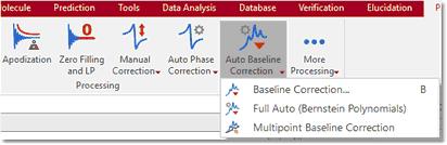
Baseline correction is an area in which Mnova is particularly strong. The software implements Manual Baseline Correction and several automatic Baseline Correction algorithms (Polynomial Fit, Bernstein Polynomial Fit and our in-house developed algorithm, the Whittaker Smoother, which gives exceptional results in 1D and 2D data sets, is extremely fast and in the vast majority of cases fully automatic and is tolerant to varying linewidths along the same spectrum and to poor signal to noise ratios). The Baseline Correction interface is also very simple. Just click on the 'Auto Baseline Correction' icon and this will execute a 'Full Auto' Baseline Correction. If you click on the scroll menu, you will be allowed to choice between the algorithms available:
Mnova will be able to import the baseline correction from the spectrometer by following the menu 'File/Preferences/NMR/Import' and checking the applicable box.
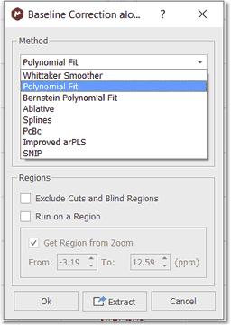
THE BASELINE CORRECTION DIALOG BOX
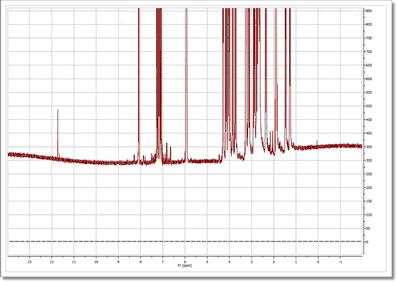
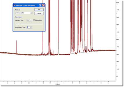
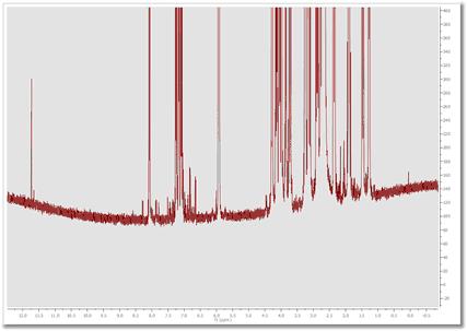
As a simple example of baseline correction, in the figure below we show a 1D spectrum in which the baseline distortions are evident. Note that the baseline not only deviates from the 0 level (represented by the gray dotted line), but it does also contain a significant rolling. You can choose the parameters of the baseline correction by dragging the parameter control (in the red circle in the 'Baseline Correction' dialog box above) or by introducing the values of the parameters directly into the edit boxes. You can also select 'Autodetect' if you prefer Mnova to calculate the best parameters for your spectrum.
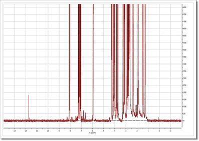
After baseline correction (fully automatic), using the Whittaker Smoother algorithm, the baseline becomes perfectly flat as depicted in the figure below
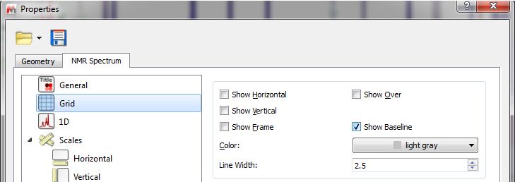
NOTE: Follow the menu 'Properties/Grid' to draw the baseline by selecting the applicable option (very useful if you have removed the vertical scale):
Whittaker Smoother Algorithm: it is a new procedure for automatic baseline correction of frequency-domain NMR data sets which we show to be highly effective on 1D and 2D spectral datasets, and which preserves the range of component line widths which are present in the sample.
The algorithm consists of two independent processes:
1. Automatic baseline recognition (signal-free regions) based on a Continuous Wavelet Derivative transform (CWT) followed by iterative threshold detection in the Power mode domain.
2. A baseline modelling procedure based on the Whittaker smoother algorithm.
Overall, the algorithm has been designed to afford perfect baselines in NMR data sets spanning a wide range of possible baseline topographies and signal-to-noise ratio (SNR) conditions. In most cases, it can be applied successfully without any operator interaction, but further versatility is assured by two parameters which could be adjusted to guarantee an optimum outcome. The procedure can therefore be ‘‘tuned’’ to achieve more accurate baseline recognition of signal-free regions, or to increase smoothness at the expense of spectral fidelity, or vice versa.
You can find more information about this 'in-house' developed algorithm in this reference: Cobas, J.C. et al. J. Mag. Res. 183, 2006, 145 and this mini review.
Polynomial Fit: In some cases, the employment of polynomial interpolations offers the advantage of smoothing the corners of each section. The user can adjust the polynomial from first to 20th order as well as the so-called 'Median Filter' (the user can see in real time the exact effect of the algorithm by a green line drawn on the spectrum display).
The polynomial used in this interpolation is:
where a1-aN are the coefficients to be fitted to the baseline and x the coordinates along the spectral axis.
Bernstein Polynomial Fit: This interpolation is defined by the following polynomial: The user only needs to select the order of the polynomial (a1-aN) and then click 'Ok'.
For a 2D example, see the 2D NMR Processing Tutorial.
Please bear in mind that you can extract the baseline correction when you are working with 1D-NMR spectra by just clicking on the 'Extract' button. Once the baseline correction has been extracted, you can use it to correct the baseline of any other spectrum by using the 'Arithmetic' feature. You can see in the picture below that we have applied the previously extracted baseline correction of the sample 'js1pmquin' to the sample named 'STANDARD 1H OBSERVE' by applying a subtraction of the spectrum minus the baseline (Spectrum-Baseline=Spectrum with Baseline Correction).
Ablative Baseline Correction: powerful algorithm for 1D-NMR spectra without negative peaks. The ablative baseline correction works in frequency domain on NMR spectra which do not have negative peaks, nor prominent negative artifacts. It works best on spectra with relatively sharp peaks (though typical “broad” labile peaks are generally not affected). It works, basically, by repeatedly “shaving off” positive peaks. Since it does it by alternating up- and down- sweeps, it is reminiscent of the carpenter’s ablative tool used to produce smooth surfaces (which is where it takes its name). The algorithm gets negatively affected by negative-pointing peaks, including artifacts (like those from saturated water). In both cases the result is an improperly handled area extending over a significant portion of the spectrum. In many cases there is nothing of interest in that area, so the result is still perfectly usable. But sometimes it disturbs, in which case one should first get rid of the undesired features. The algorithm gets also affected badly by Bruker smileys. Because of that, 2% of the spectrum on both ends are always set apart and considered as their own baseline. The result is that in the final spectrum, they get cut off.
Splines: it uses smooth curves to link the points. This method comprises two stages: First, it uses an algorithm that detects signals-free regions which are then connected, in a second stage, with splines to build the baseline model which is then subtracted from the original spectrum.
PcBC: this is an experimental method that works by simultaneously correcting the phase and baseline of a 1D spectrum. While it can be used for both purposes, it can also be applied.
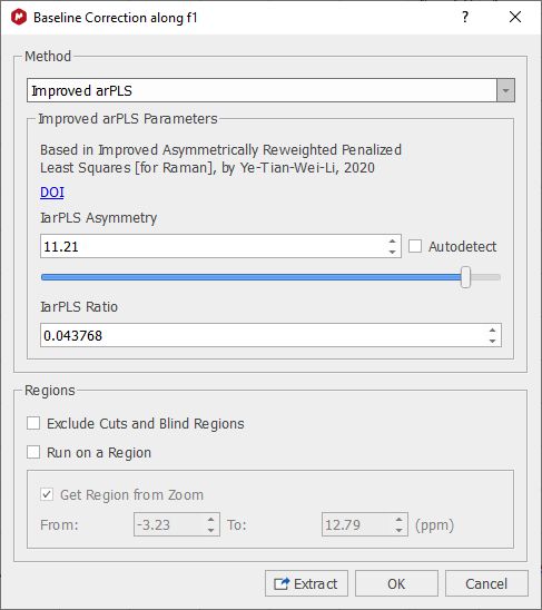
Improved arPLS: a baseline correction method based on improved asymmetrically reweighted penalized least squares.
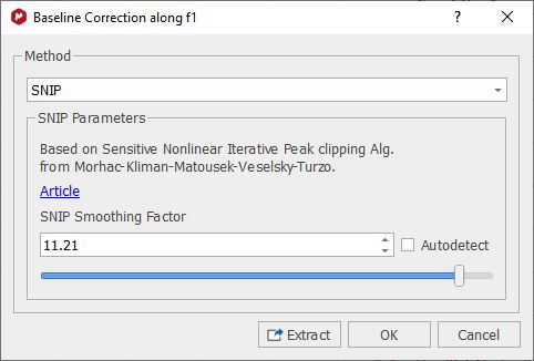
The algorithm is very sensitive to the presence of downward pointing peaks (this may limit its applicability to poorly phased NMR spectra). It has an internal step (z-scores) that attempts to ignore sharp downward spikes when computing the baseline. Note that this may not work for not-too-sharp downward peaks. The "ratio" parameter is set to 1e-6. This value should work for most situations, and should not approach 1e-1 except for some 2D cases for which the number of iterations (limited to 50) are to be kept as low as possible for speed reasons. Otherwise relatively large values may lead to nonsense results. The Log10(lambda) parameter modulates how closely should the baseline follow the spectrum values (not its "stiffness"), and is intended to be tuned by the user for each particular case. This algorithm is based in this one (implemented for Raman): https://doi.org/10.1364/AO.404863 SNIP: Sensitive Nonlinear Iterative Peak baseline correction algorithm has been implemented based on this paper.
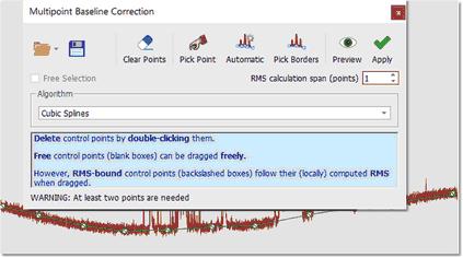
Multipoint Baseline Correction: This method provides a way of modeling the baseline by selecting a well-distributed set of points that fall on the baseline and then interpolating between those points to complete the model. Please keep in mind that this method is not scriptable and can not be included in the Processing templates.
The following spectrum shows significant baseline distortion:
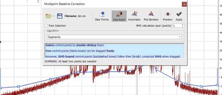
Next, select the 'Multipoint Baseline Correction' under the 'Auto Baseline Correction' scroll down menu. This will display the 'Multipoint Baseline Correction' dialog box which will allow you to put down points along the baseline (by clicking on the 'Pick Baseline points' button
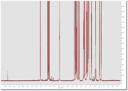
After subtracting the estimated baseline model, this is the resulting spectrum:
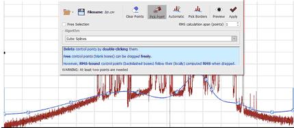
Let´s see the functionality of each button of the ''Multipoint Baseline Correction' dialog box: 'Load and Save': to import and export multipoint baseline correction settings and points. 'Pick Baseline points': allows the user to pick the points. To remove any selected point (highlighted in green), just double click on it. 'Automatic' automatically add points for the baseline correction 'Pick Borders': allows the user to pick the first and the latest points. 'Clear all baseline': click on this button to delete all the selected points. 'Toggles Preview Showing': to see a preview of the baseline correction. 'Apply Baseline Correction': to apply the correction. 'Free Selection' : to pick a point anywhere. 'RMS Calculation span (points): The multipoint baseline algorithm builds a baseline model using the points selected; but if you select this option; instead of use the specific points selected in the spectrum when clicked, it uses an average value calculated from the point and the surrounded points given by the "average window" value. For example, and average window of 0 will use exactly the clicked/selected point, and a average window of 2 will use the average of the clicked/selected point and 2 point from the left and 2 points from the right, ie, in total it will use 2*n+1 points where n is the average window 'Algorithm': from this drop down menu, we can select the algorithm for the baseline correction: Segments: it simply connects the points with flat lines. This baseline will not be smooth, it just abruptly links the points with segments.
Cubic Splines: it uses smooth curves to link the points
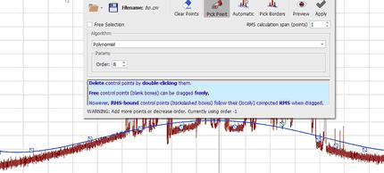
With segments and splines the baseline go thorough all the points defined by the user. This will not happen with the remaining algorithms: Polynomial: the baseline will be adjusted to a polynomial function
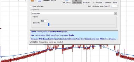
Witthaker: it will use the Witthaker Smoother algorithm to fit the baseline.
NOTE: After having applied a baseline correction in a 2D dataset, the manual phasing could be greyed out. To undo the baseline correction, follow the menu "Processing/Processing Template' and turn off the Baseline Correction for either dimension, click on OK and you will be able to correct the phase manually. |