Zero Filling and Linear Prediction

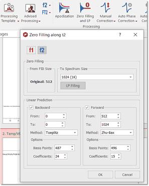
Zero Filling: This option can be used to set the size of the Fourier Transform. It can be used either to increase the digital resolution or to truncate the FID. When the time-domain signal is subject to a FT, the resulting spectrum is represented by a set of data points (by joining the points to plot the spectrum as a smooth line). As a Fourier transformation preserves the number of data points, if we take the original FID and add an equal number of zeroes to the end of it, the applicable spectrum will have double the number of points, increasing therefore the 'apparent' digital resolution of the spectrum. The zero filling process is equivalent to a frequency-domain interpolation. This command is available in the Processing ribbon:

Mnova will be able to import the Zero Filling and Linear Prediction from the spectrometer by following the menu 'File/Preferences/NMR/Import' and checking the applicable box.

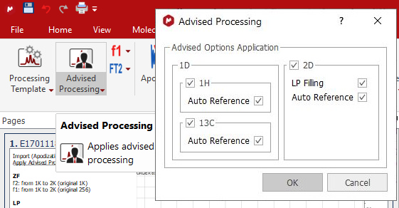
There is also an 'Advised processing' feature which will apply a suggested processing with the option to automatic reference the spectra and to apply a Linear Prediction:

For 1H it will apply a Stanning apodization of 4.0 and a three fold Zero Filling. For 13C datasets, it will include an exponential apodization of 2.0 Hz (on top of the Stanning).

For 2D, it will apply a Zero Filling along F2 with a maximum factor of 2 and an exponential apodization of 2.0 Hz and Stanning 4.0 and a 'Fit to Highest Intensity'

For F1 it will apply a Sine Square 90º (first point: 0.5) apodization and a ZF (up tp 3 times).

Magnitude phase correction (only in f2) will be also applied in case of HMBC spectra an in other 2D spectra where FT is None. 

In other cases, Regions phase correction will be applied in both F1 and F2.

In some cases, the FID does not fulfill the requirement of the number of data points corresponding to an entire power of 2. In these cases, Zero Filling must be applied to the immediately higher entire power of 2 for FT to be possible. Mnova will automatically carry out this Zero Filling when the number of data points is not an entire power of 2. By default, Mnova proposes a duplication of the original number of FID data points. For example, if the FID has 16384 data points (or a number of data points between 16385 and 32768), the Zero Filling open dialog would show us the value of 32768 (32K) data points, which indicates that Mnova will add up to 16384 data points at the end of the FID.

Linear Prediction (Not available in Mnova Lite): Linear prediction is a mathematical procedure where a missing part of a FID can be constructed in order to increase the digital resolution of the spectrum; it is a tool which examines the free induction decay, extracts a set of coefficients, and extrapolates, either forward or backward, to predict what the data would have been had it been collected. This is a potentially valuable technique for extraction of useful information from marginal data.

Linear prediction is based in this fundamental principle: each value in the time series can be represented as a linear combination of the immediately preceding values. Mathematically, the basic LP equation postulates:

where ap are the LP Coefficients and the number 'p' corresponds to the order of the prediction. Thus, you can extrapolate the series beyond the point N. This equation is known as Forward Linear Prediction (extrapolates forward, predicting the new values from the older ones).

Backward Linear Prediction will be represented in the following equation:

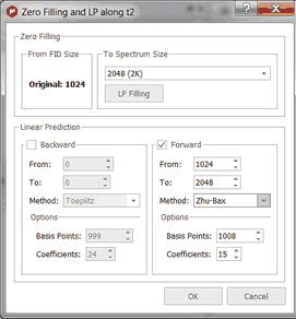
This command is available in the same menu as zero filling. If you need to repair the baseline distortions (due generally to the first points of the FID) you have to tick Backward LP and select the limits; this will predict the first points of the FID.

Forward Linear Prediction is a better alternative to correct the last part of the FID than zero filling; this will extrapolate the FID in the direction of the advance, predicting the new data points from the older. If you select 'Linear Filling', a Forward LP  from the end of the original FID up to the number of points defined in the ‘Spectrum size’ combo box, will be executed. You can also set the number of Basis Points and Coefficients of the algorithm that you want to use for Linear Prediction.

Method: Linear Prediction is extremely useful in 2D NMR as a way of reducing the acquisition time or increasing the quality of already existing data sets. Also, in 1D NMR it is useful when the FID has not decayed to zero before experiment completion. This often happens when working with slowly relaxing nuclei (such as quaternary carbons, in 13C-NMR) and in experiments with a wide ppm area (spectral width).

One of the most common causes of the corruption of the first data points of the FID is the security time or pre-scan delay (time which exists between the pulse and the beginning of the acquisition) which in many cases may not be enough to allow the detector to recover fully from the effect of the pulse.

Our LP implementation is based in a very fast orthogonalization of Toeplitz matrices which is one of the fastest implementation of LP algorithms used in NMR. It gives very good results with phase sensitive data, in particular with HSQC and related spectra. However, it does not work very well with spectra in magnitude (or non phase sensitive) mode. In fact, Toeplitz method does not make it possible to reflect the roots of the LP coefficients within the unit circle because the resulting new LP coefficients get worse.

With such problems in mind, we decided to try the well known Zhu-Bax approach. In short, the algorithm calculates the forward and backward LP because in theory they should be identical. However, in presence of noise they are different. Zhu and Bax proposed to reduce the contribution of the random errors induced by noise by simply averaging the two sets of coefficients (fwd & bwd). Finally new roots are computed based on the average coefficients.

Zhu-Bax LP algorithm has been speeded up and it will be the default algorithm for forward LP as it is numerically much more stable and produces more artifacts-free spectra.

The Burg method is probably the first implementation of Linear Prediction developed by John Burg many years ago and it was extensively used in geophysics, but in general, should not be used with NMR data.

 Coefficients: number of theoretical sinusoids. The number of the coefficients should be equal to the number of points in the FID in an ideal case. By default Mnova sets the number of coefficients according to:

 Number Of Coefficients = points in the spectrum/16

 Basis Points: they are the number of ‘good’ experimental points to be entered in the calculations. The number of basis points should be at least twice or three times greater than the number of coefficients.

MIST: This option is aimed at extending the FID using a modified Iterative Thresholding algorithm. Its performance has not been studied thoroughly so its application must be used with caution.

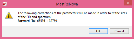
If some LP parameters don't match the sizes of the FID and spectrum then instead of auto-fitting them, a message box with the suggested corrections will be appear: