Apodization

Apodization (or Weighting or Windowing): literally, apodization means 'cutting off the feet' in the original Greek. In this case, the feet are the leakage or wiggles which appear when the signal decays rapidly to zero producing an abrupt truncation of the FID, as can happen for example when zero filling. Apodization is a very useful approach to enhance the S/N ratio (sensitivity) or the resolution, or even to remove truncation artefacts, after data has been collected.

The most commonly used apodization function is a decaying single-exponential curve. The magnitude of the decay constant determines how quickly the curve decays. In a regular FID, the resonances due to the sample are found in the earlier parts of the signal. When you multiply the FID by a decaying-exponential function, you favour the early parts of the time domain and attenuate the data at the end of the acquisition period, which is essentially all noise. A single exponential apodization function does not significantly affect the signal at short times, but it greatly reduces the noise at later times; at the expense of an increase in linewidth, that is to say, a decrease in the resolution. On the other hand, if you use an increasing exponential curve as apodization, you will obtain finer lines (increased resolution) but amplifying the noise (decreased sensitivity).

The Window function is applied by multiplying the data vector d, element by element, by a vector a. Thus element k of vector d is multiplied by element k of vector a to yield element k of vector d'.

 d'k= akdk

The challenge lies in finding a vector a, such that the noise in the tail of the FID is attenuated without excessive line broadening or, in the case of apodization, to smooth the truncated data exponentially towards zero, again without excessive line broadening. Theory shows that this is attained when the decay of vector a matches the decay of vector d; in this case we have what is known as a matched filter. Mnova makes this particularly easy by allowing the final spectrum to be observed while the decay parameter of the window function is adjusted.

Mnova incorporates many window functions (Exponential, Gaussian, Sine Bell, Sine Bell Square, TRAF, Trapezoidal, Parabolic, Hanning, Convolution Difference and Linear Ramp), which can be combined and can be used interactively (while viewing the FID as well as the resulting spectrum) to improve the sensitivity or the resolution. Unfortunately, it is very difficult to find a function which improves sensitivity and resolution simultaneously (an exception could be the Traficante function, as we will see later).

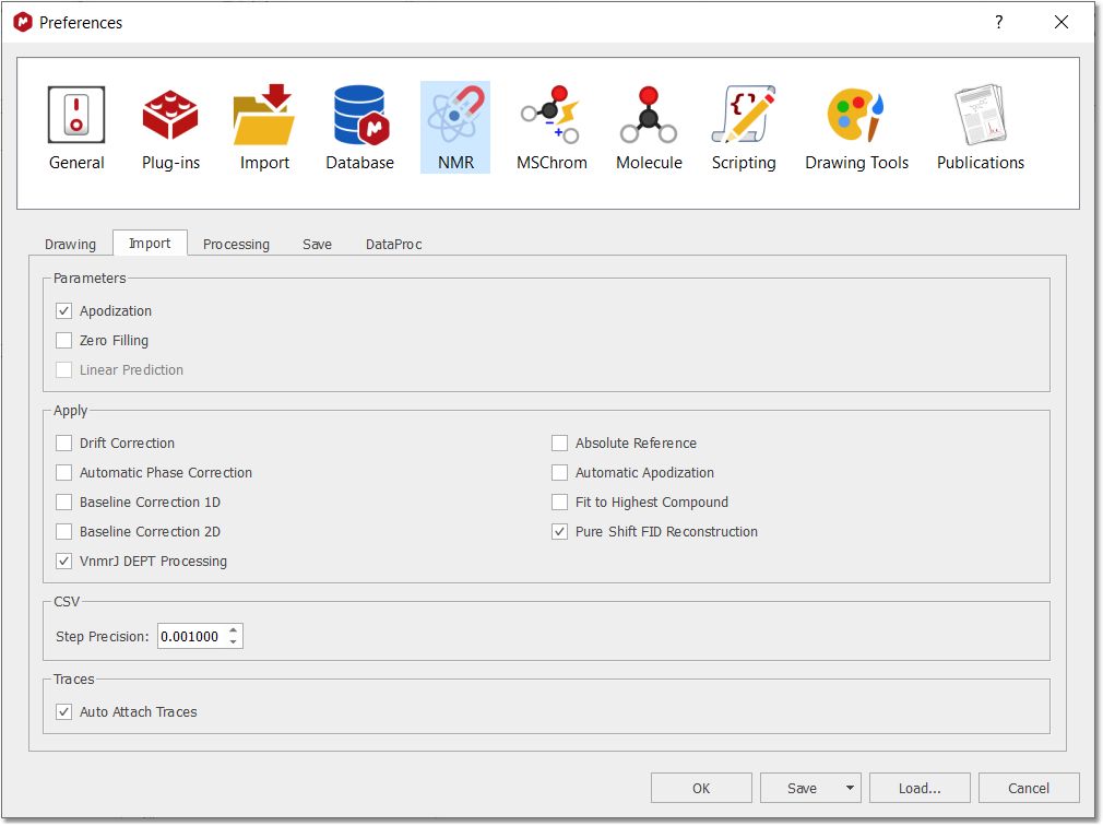
You can import the apodization used in the spectrometer by following the menu 'File/Preferences/NMR/Import':

You can also let Mnova to apply an Advised Processing by clicking on the applicable button of the ribbon. In that case, Mnova will apply Stanning apodization of 4.0 in 1D (and for 13C it will add an exponential apodization of 2.0 Hz). For 2D, it will apply an exponential apodization of 2.0 Hz and Stanning 4.0 if F2 and Sine Square 90º (first point: 0.5) in F1.

The apodization feature can be found in the Processing ribbon (shortcut: W):

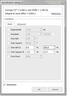
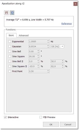
Once you have selected 'Apodization', a modeless dialog box will be displayed:

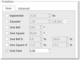
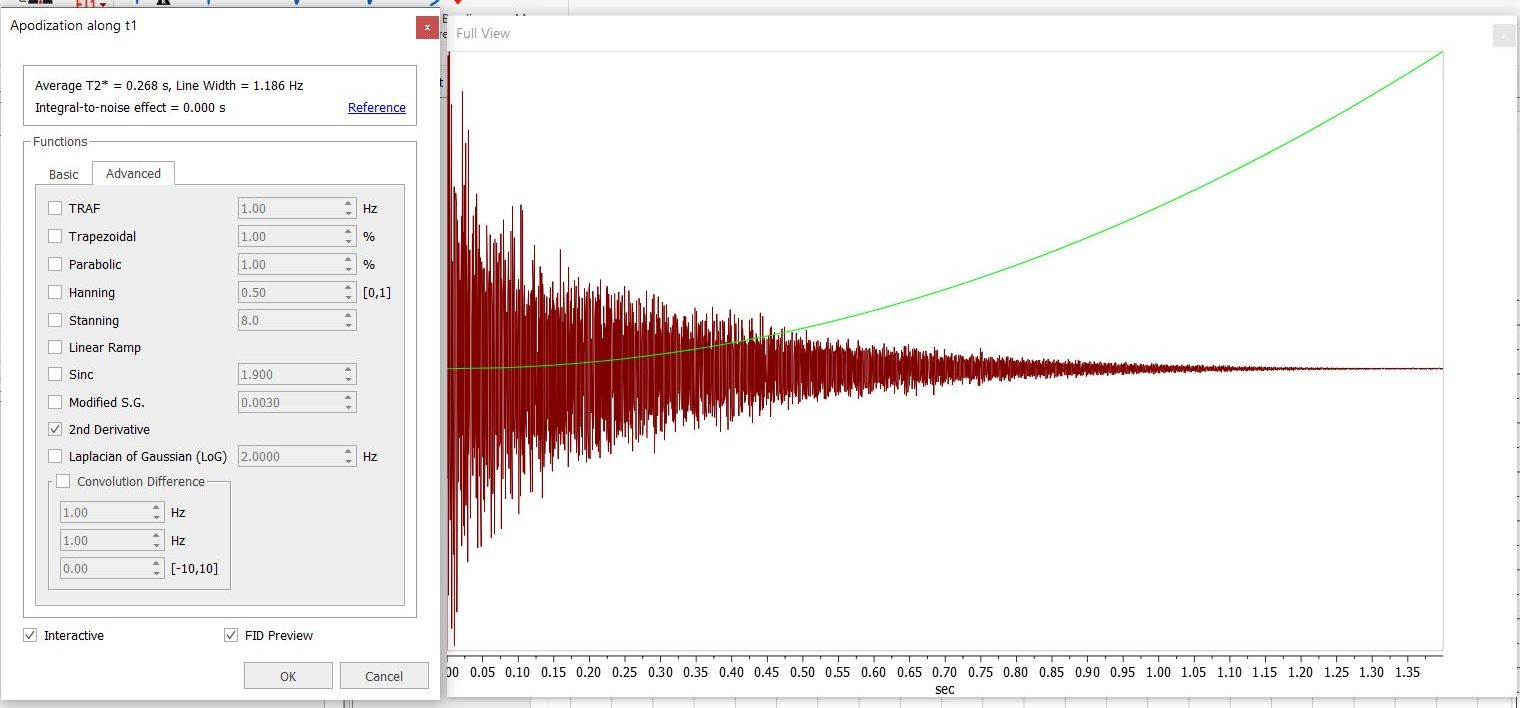
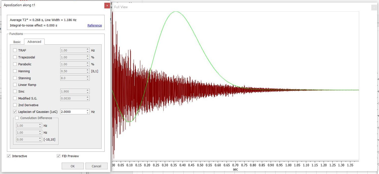
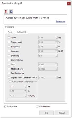
As it is a modeless dialog, you can change the intensity of the spectrum while the dialog is open. In 2D-NMR spectra, you will be allowed to switch from F1 to F2 to select the desired apodization function.
 

In this dialog box you will find the type of window function which Mnova has applied prior to FT, as well as other Standard Functions (Gaussian, Sine Bell, Sine Square and First Point). If you select the 'Advanced' tab, you can set other apodization functions, as shown below:

In order to assist in the process of finding the most suitable window function and its parameters, Mnova allows the user to interactively adjust the parameters of window functions, and to view the effect directly on the frequency spectrum. For this purpose, make sure the 'Interactive' box is ticked, you can then follow the exact effect of the function you are applying on the frequency domain spectrum (or on the FID, if you are on the FID' view) by using the buttons to change the desired parameter. If you have checked the 'FID preview' box or activated the 'Full View' window (by holding down the F2 key or by checking the applicable box under the View ribbon) you will be able to see the window function displayed along with the FID.

.

We will try to explain in a brief and easy way the applications and the effects of these functions:

Exponential: A exponential apodization function is defined as:

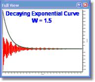
                         ak = e-πWkΔt

where W (the parameter to adjust) represents the the line broadening factor expressed in Hz. So, if the original width of the signal is 'L', the final width of the signal after applying this window function would be 'L+W'. If W is positive we will have a decaying exponential curve (and we are giving more weight to the points at the beginning of the FID and suppressing the data at the end of the time series, which is essentially all noise). As we explained previously, this will increase the 'sensitivity' (Signal to Noise Ratio) of the spectrum at the expense of an increase in linewidth (decreased resolution).

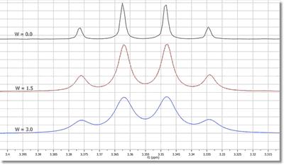
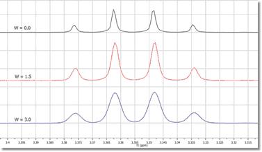
The figure below shows the effect of W on the linewidth. The black trace has no window function applied. The red trace shows a taller signal due to application of an Exponential Function and also an increase of the Signal to Noise Ratio (matched filter), while the blue trace shows that if the Exponential Function is too severe the broadening of the lines reduces the signal size again.

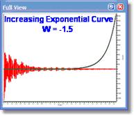
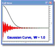
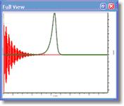
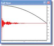
If W is negative, we will have an increasing exponential curve, thus obtaining the opposite effect (increased resolution, with finer lines, and a decrease in sensitivity, i.e., a lower S/N ratio). You can see below the graphical difference between an increasing and a decaying exponential curve over the FID (shown in the 'Full View' window). Note that in this case an increasing exponential curve will not be a good choice (it is normally used in combination with other functions, such as Gaussian).

In most of the literature this parameter is symbolized by LB (Line Broadening).

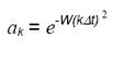
Gaussian: In Gaussian window function resembles the Gaussian Probability Distribution function used in statistical analysis. The gaussian function rises quasi exponentially to its single maximum and then falls back to zero in the same manner and so may be regarded as almost two back-to-back exponentials.

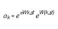
In Gaussian apodization, each data point of the FID is multiplied by the vector:

where W is the same widening factor used in exponential apodization. This function is similar to the exponential but decays comparatively slowly at the beginning of the FID and then quite rapidly at the end. For this reason, it causes less line broadening than the exponential multiplication.

In the next picture, you can see the influence of W over the linewidth:

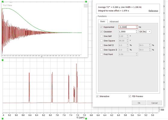
Gaussian plus Exponential: This function is also known as Lorentz-to-Gauss Transformation and is not directly implemented in Mnova, but you can apply it by ticking both exponential and Gaussian multiplication functions and introducing a negative value for the exponential line broadening (W) and a positive value for the Gaussian parameter (GB). The spectrum can be optimized for resolution by suitably adjusting these parameters.

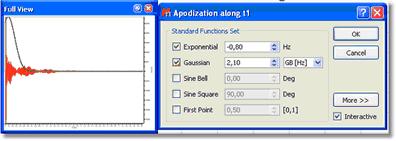
Thus, this weighting function combines a rising exponential function with a decreasing Gaussian function; then, the resulting vector will be:

To perform Exponential/Gaussian apodization with Mnova, select the Apodization option in the FT scroll menu on the toolbar, then click on the Exponential as well as on the Gaussian resolution enhancement option and finally enter the appropriate values of W (or LB) and GB and click OK.

Usually, a process of trial and error is adopted with the parameters being adjusted until the best result is obtained. You can follow (by ticking on the 'Interactive' box) the exact effect of the function you are applying on the frequency domain spectrum or on the FID window (shown graphically in the 'Full View' window), as you can see in the screenshot below.

GF (Gaussian Factor) is a number between 0 and 1 and defines where the maximum of the function will be, as a fraction of the acquisition time.

Sine Bell (Not available in Mnova Lite): This function is very useful in those NMR experiments where the signals of interest are not maximal at the beginning of the FID and very convenient for magnitude spectra because it reduces the dispersive part of the line shape.

In COSY experiments the cross peaks are sine modulated while the diagonal peaks are cosine modulated. Sine bell windowing thus emphasizes the cross peaks and attenuates the diagonal signals. Unfortunately due to differing relaxation times for some signals possibly not all cross-peaks will be maximal at the same time; in this case the sine-bell may be shifted to yield the best compromise spectrum. The unshifted sine-bell also removes dispersive signals from the absolute value COSY, providing the sought for absorption line shape.

Avoid using this function with 1D spectra since it decrease the spectral intensity. If used with phase sensitive experiments the sine bell can result in signals with negative side lobes and near zero integrals.

This function consists in the multiplication of each data point of the FID by the next vector:

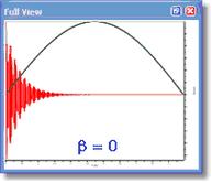
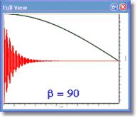
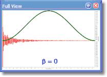
Mnova requires you to enter the β parameter, whose input is expressed in degrees. When β = 0; the equivalent function is a sine-bell, while when β = 90 the equivalent function is a cosine-bell. In the pictures below you can see the representations of the sine bell functions resulting from different values for β:

The cosine-bell apodization (β = 90) is very convenient in 2D-HSQC experiments:

You can use the "VNMR-like version of sinebell apodization" which uses % of acquisition time (instead of seconds) in order to make the parameters applicable to other spectra with the saved processing template.

The full formula for the shifted Sine II is sin(((t - sbs)*pi)/(2*sb)).

Where sbs = sbs Mnova /100*T AQ; sb = sb Mnova/100*T AQ

For function values less than zero, the function is truncated (i.e., only the first set of positive values are used).

As you can see you can also adjust the time-period of the SineBell (like the "sb" parameter in VNMR)

Sine  Square (Not available in Mnova Lite): The shape of  the Sine Bell weighting function is altered by squaring it, resulting on the Sine Bell Squared function, which is more concentrated over the maximum. It is very useful to use a 90° shifted sine-bell squared to apodize 2D phase-sensitive experiments.

First Point Correction: There is an important difference between the discreet FT and the continuous FT. The discreet FT generates a constant vertical displacement of the baseline, which can be due to a distortion of the first point of the FID. It treats the FID as a function which is repeated periodically, thus the ordinate at t=0 would represent the algebraic average of the first and the last point. In most FIDs, the value of the last point is very close to zero, and thus the first real point would have to be divided by two, before introducing it in the FT algorithm. It is often necessary to multiply the first point of the FID by 0.5 before FT in order to ensure that the value of the integral over the spectrum is equal to the value of the first point of the FID.

You can alter this multiplication parameter by entering the desired value (it should be 0.5 by default, as you can see in the FT dialog box below).

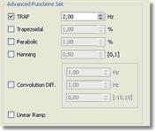
The functions which follow are accessed via the [More >>] button in the Apodization dialog box.

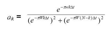
Traficante (Not available in Mnova Lite): The Exponential Multiplication Gaussian and the combination of both can improve spectral resolution at the expense of some loss in SNR. The Traficante window function endeavours to improve resolution without noticeable loss in SNR. Traficante enhances the middle part of the FID and then uses a matched filter to attenuate noise in the latter part of the time-series. The process involves the division of the FID by the sum of the squares of the FID and its reverse. If there are N data points, the kth point in the original FID is point k while the applicable point in the reversed FID is point (N-k). As the resulting FID is symmetrical (with respect to the midpoint), we can multiply it by a function to obtain a new desired FID which does not decrease.

So, if we named the original FID E, and the reversed FID ε, we would get:

         E·g(t) + ε·h(t) = 1

And Traficante apodization will consist of the multiplication of the FID by the following vector:

In the picture below, we can see a Traficante function represented (with W = 2) applied to the FID

Trapezoidal (Not available in Mnova Lite): This function multiplies the FID by a trapezoidal shaped function;

where T is the acquisition time and k is the percentage of the total length of data

This option is useful to avoid the "sinc" artifacts resulting from truncation of the FID. You can select the percentage of the total length of data between 0% and 100% (k), in the advanced functions of the FT menu.                

Parabolic (Not available in Mnova Lite): This function multiplies the FID by a parabola shaped function, where  

You can also set the length of the parabola by selecting (on the FT scroll menu) Apodization, click "More", select parabolic and then choose the  desired value for the parameter (b, expressed as the total length of data). Again, you can see the exact effect of the function you are applying on the frequency domain spectrum or the effect on the the FID by (pre-)selecting the Full View" window:

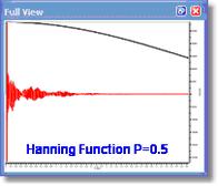
Hanning (Not available in Mnova Lite): Mnova adopts the following generalized equation:

where T is the acquisition time, and P can be a value from 0 to 1. You can set this parameter on the advanced Functions set of the FT dialog box. If P = 0.5 we will have a Hanning function and if P = 0.54 we will apply a Hanning function, producing 10 and 20% line broadening respectively. The Hanning window, more correctly called the Hann window and the Hamming window are part of a family of functions known as "Raised Cosines" and also includes the Gaussian Window. These functions, like a cosine bell, have a maximum value; Mnova generally implements these functions with their maxima at zero time. The Hanning Function is sometimes used to reduce aliasing. Aliasing arises when signals are insufficiently sampled (violating the Nyquist Criterion), resulting in spectral folding. It results in peaks appearing at incorrect positions and generally not phasing along with the authentic signals. This arises due to incorrect experimental set up (signals beyond the high frequency end of the spectral width), and the ability to correct for it after acquisition is useful indeed.

Convolution Difference (Not available in Mnova Lite): This weighting function multiplies the FID by :

where LB is the line broadening and SW is the spectral width in Hz. You can also access this function from the scroll menu of the FT icon where you will be able to set the value of LB.

Linear Ramp (Not available in Mnova Lite): This command is used to multiply the data points of the FID by an increasing linear ramp, resulting in the first derivative of the Fourier transformed spectrum { d(intensity)/d(frequency) }.  This emphasizes the faster rising parts of the spectrum at the expense of SNR. If the initial spectrum had an excellent SNR this function can dramatically improve resolution.  Mnova will soon offer derivative performed using wavelet processing which produces even better spectra.

This weighting function gives more weight to the end of the FID, amplifying the noise (decreasing the sensitivity), and for that reason we recommend its use only in combination with another function which gives more weight to the beginning of the FID (increasing sensitivity). In practical terms, add the ramp function to a spectrum that has already been windowed by, for example the EM function for 1D or the sine-bell function for a 2D in order to improve the selectivity.

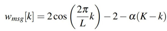
Modified Savitzky-Golay (in the time domain) Recognising that the Savitzky-Golay window is zero at the start of the signal, we propose to add a decreasing ramp to it. That is the modified Savitzky-Golay window becomes:

where α is the weight of the ramp. The larger α is, the more we weight the original signal and the higher the SNR gain will be at the expense of worse resolution enhancement.

Second Derivative: as an extension to the existing first order (that was already implemented years ago and that consists of the application of a linear ramp).

The Laplacian of Gaussian The second derivative window is of the form w2[n] = k2