DOSY/ROSY Transform


DOSY/ROSY Transform |
|
|
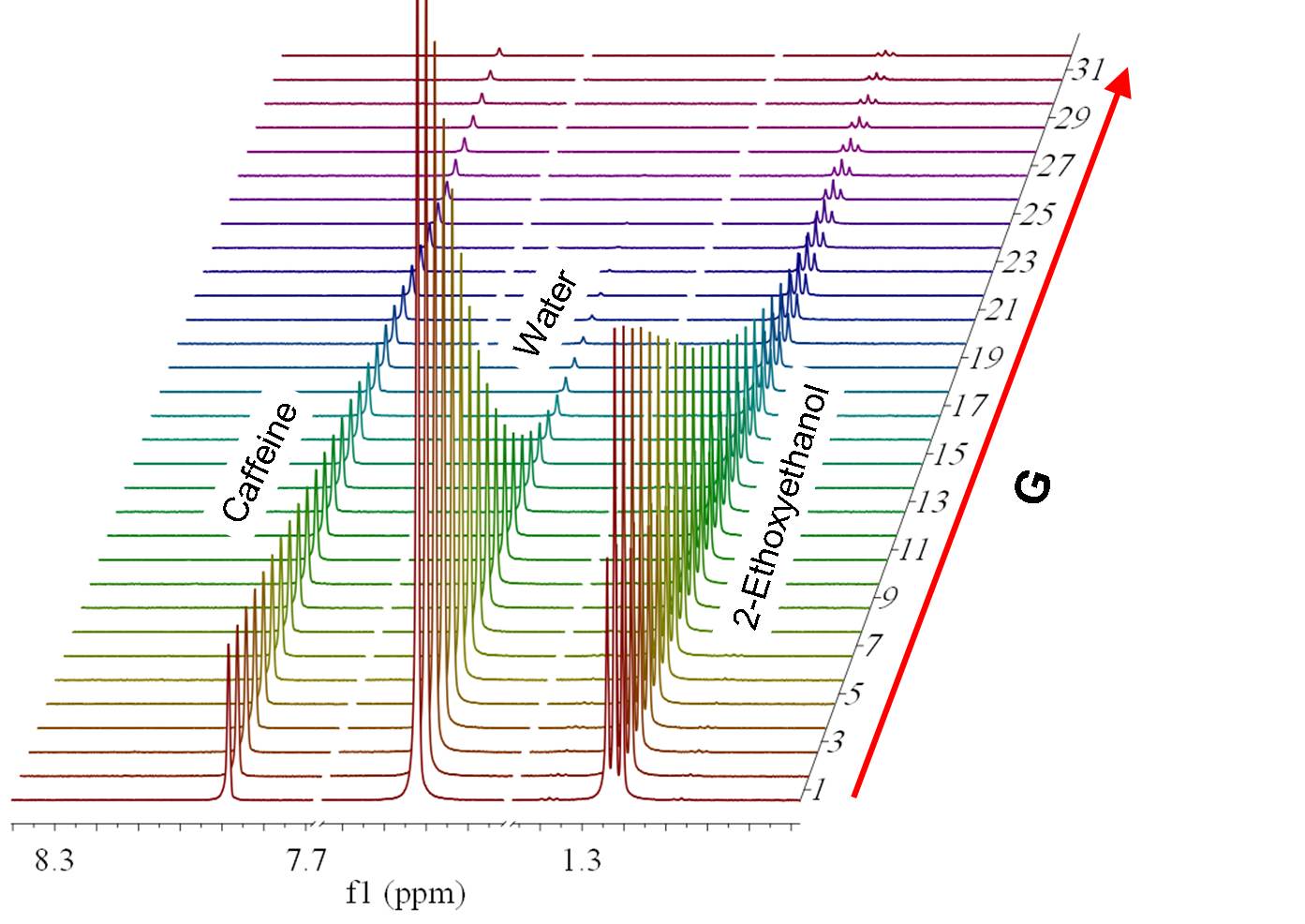
(Not available in Mnova Lite) NMR diffusion experiments provide a way to separate the different compounds in a mixture based on the differing translation diffusion coefficients (and therefore differences in the size and shape of the molecule, as well as physical properties of the surrounding environment such as viscosity, temperature, etc) of each chemical species in solution. In a certain way, it can be regarded as a special chromatographic method for physical component separation, but unlike those techniques, it does not require any particular sample preparation or chromatographic method optimization and maintains the innate chemical environment of the sample during analysis. The measurement of diffusion is carried out by observing the attenuation of the NMR signals during a pulsed field gradient experiment. The degree of attenuation is a function of the magnetic gradient pulse amplitude (G) and occurs at a rate proportional to the diffusion coefficient (D) of the molecule. Assuming that a line at a given (fixed) chemical shift f belongs to a single sample component A with a diffusion constant DA, we have Please note that loading a stacked plot of 1D NMR spectra will also display the result in the 3D viewer:
Bayesian DOSY Transform Let´s see how this feature works step by step: 1. Import your raw data: for example by dragging the spectrum folder into Mnova:
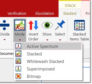
2. Process the spectrum: Mnova processes the spectrum automatically for you. However, it might be necessary to apply some further processing, usually manual phase and baseline correction You can do that directly on the stacked plot mode, but it’s recommended to use the ‘Active Spectrum’ mode as depicted below:
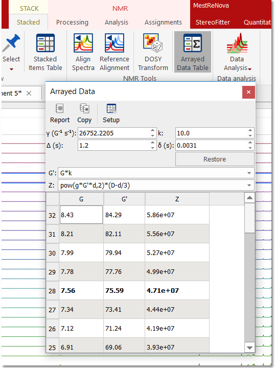
Within the ‘Active Spectrum’ mode, correct any phase distortion and apply an automatic baseline correction (use Berstein polynomials). These corrections will be applied to the whole dataset. You can also apply the Align tool (under the Stacked ribbon) if the traces are not aligned. 3. Setup Diffusion-related exp. values: Make sure that the big and little delta values have been correctly read from the experiment files by following the menu 'View/Tables/Arrayed Data' (or Stack 'Arrayed Data Table').
These values should be entered in seconds:
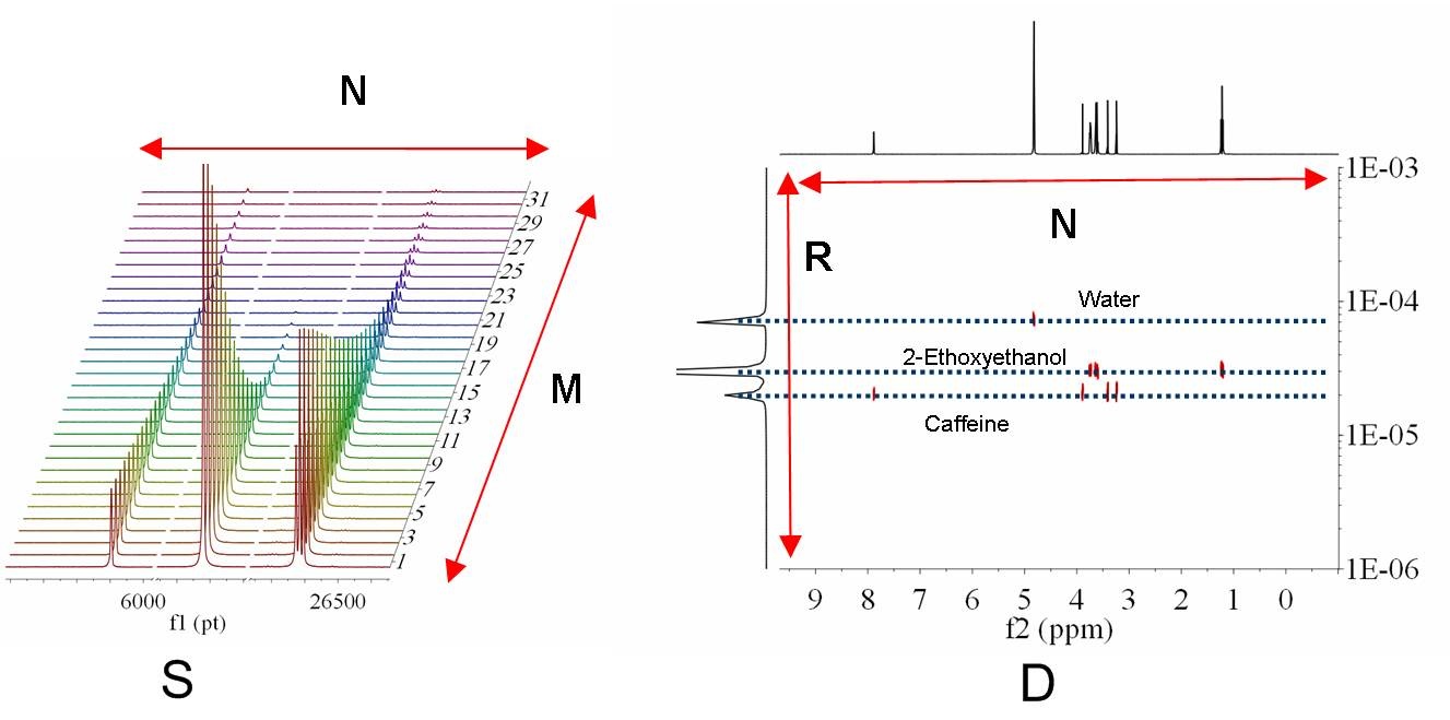
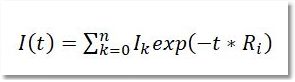
By means of the bayDOSY transform (BDT) we are fitting a model of the type S(f,z) = SA(f) exp(-dAz) where SA(f) is the spectral intensity of component A in zero gradient (‘normal’ spectrum of A) and dA is its diffusion coefficient. Z values corresponding to the expression above are displayed in the third column which are calculated according to the formula highlighted in the figure. It’s assumed that the gradient strength comes in G/cm. Note that the values used by the algorithm are those listed in the G’ column which are in turn obtained from G column after multiplying these values by the k factor.
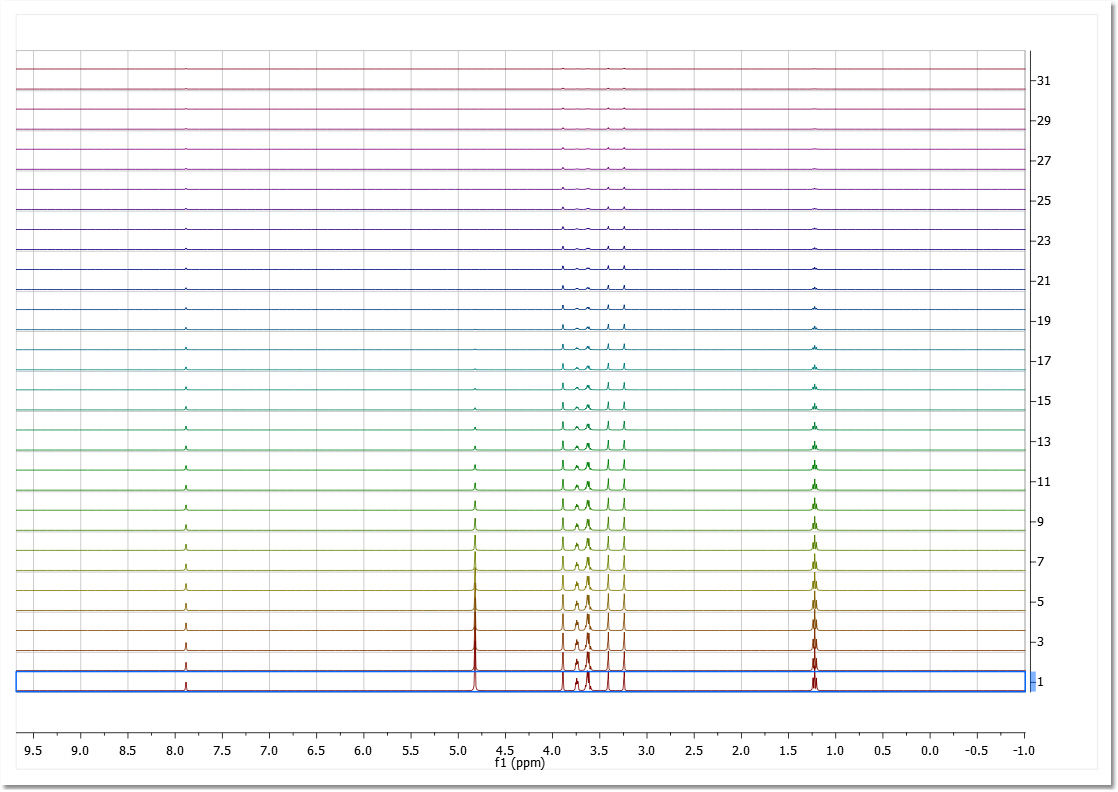
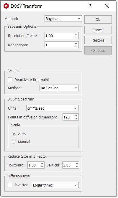
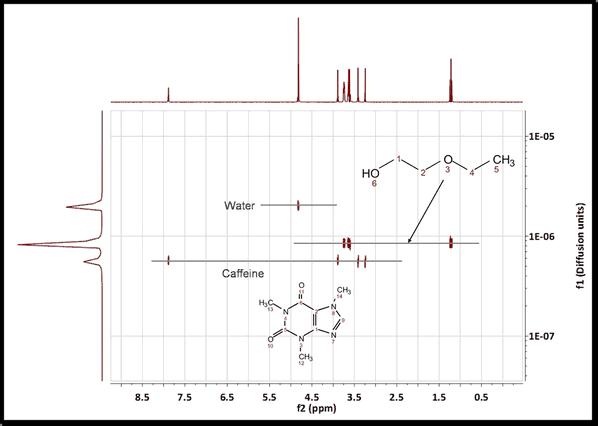
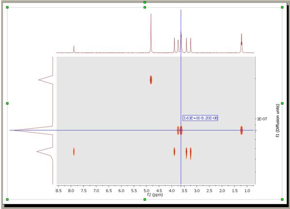
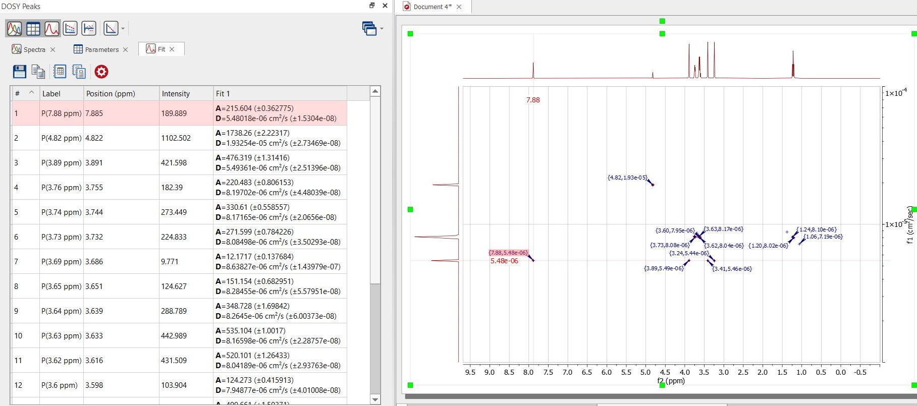
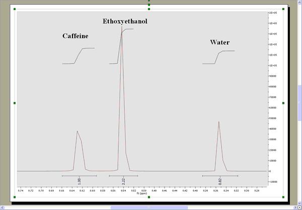
4. Run the DOSY Transform: Just by following the menu 'Stacked/DOSY/ROSY Transform' a) To start with, use a resolution factor of 1 (or 0.1). Higher values will increase the resolution along the diffusion dimension (vertical). However, small peaks can be missed when the resolution factor is too high b) The number of repetitions should be kept to 0 for the first try. Next, if you want to further increase the vertical resolution, set this value to 1 or 2. This should drastically increase the resolution, though some artifacts might appear. c) Scaling: you can apply 'no scaling', 'scale consecutive' or 'scale halves'. Scale Consecutive: it is often used in experiments where big delta is varied and serves to minimize the influence of T1 relaxation to the data. Scale Halves: only the first half of the spectral set in the stack is shown in the result. Check the 'Deactivate first point' box if you want to discard the first spectrum of the stacked plot, making sure that you end with an odd number of traces. d) If the gradient strengths have been introduced in G/cm, the resulting diffusion coefficients will be in cm^2/s.Those units could be also changed under the 'Properties' dialog box (or by right clicking on the diffusion scale of the pseudo 2D plot) This is the result obtained. As you can see the 3 compounds (water, ethoxyethanol and caffeine) are perfectly separated.
You can use the 'Crosshair' to measure the Difussion values.
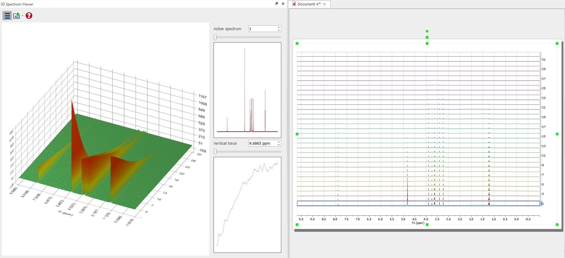
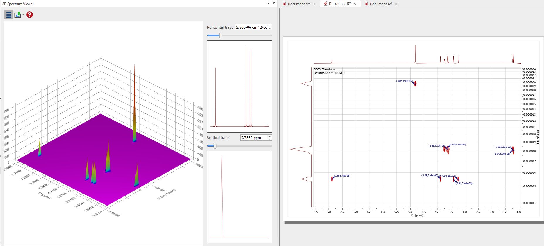
The result can be displayed in the 3D viewer:
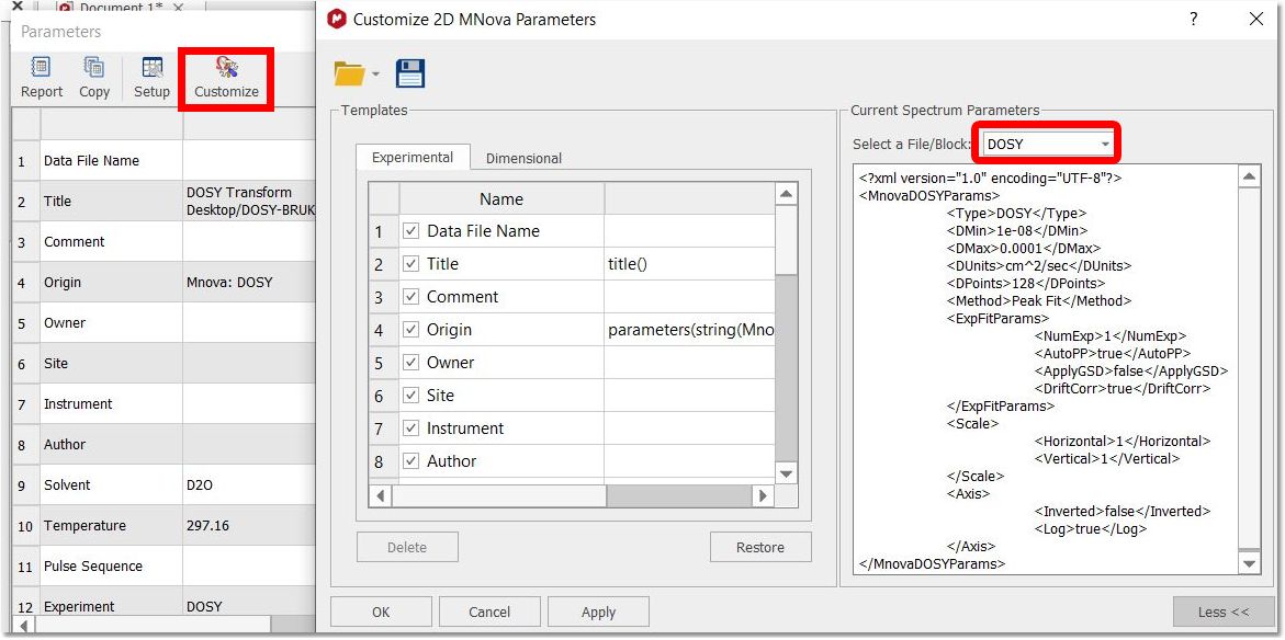
You can check the setting used for the DOSY transform by following the menu 'View/Parameters/Customize' and selecting DOSY block from the scroll down menu:
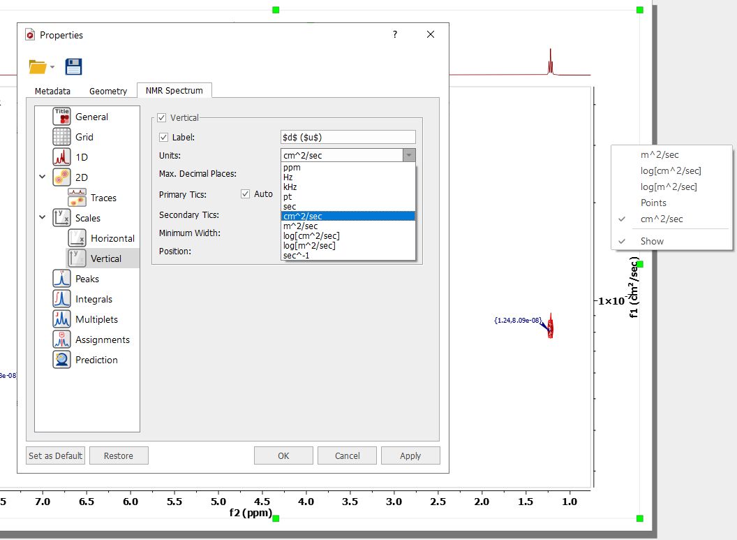
The diffusion units can changed under the 'Properties' dialog box (or by right clicking on the diffusion scale of the pseudo 2D plot):
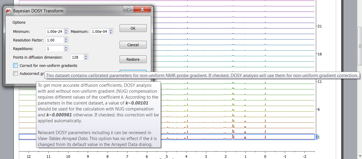
Non-uniform gradient (NUG) correction can be applied by checking the option "Correct for non-uniform gradients" in Bayesian DOSY Transform dialog (the options only appear if the dataset requires them):
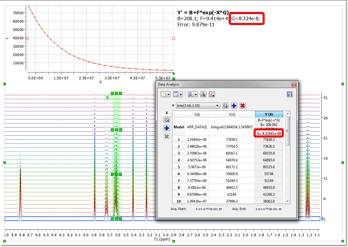
You can also use the 'Data Analysis' feature to get your Diffusion coefficient in the traditional way (given by the value of the parameter G):
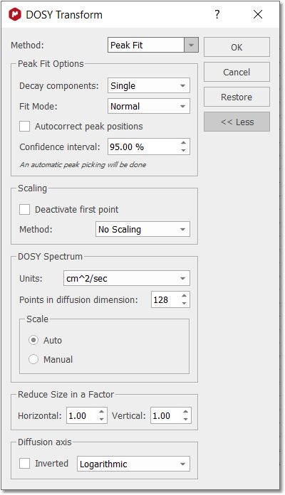
You can display the diffusion axis in logarithmic scale (even with vertical scale inverted), just by checking the applicable options obtained after having clicked on the 'advanced' button. Peak Fit Method The "Peak Heights Fit" method was added to DOSY processing capabilities. The existing Bayesian DOSY routine provides a full continuous map of diffusion coefficients found in the system. To provide a more "filtered" DOSY 2D output and improve consistency with other spectrometer software a new DOSY processing technique is implemented.
After data preparation the Peak Fit method fits the extracted peak intensity values using exponential decay. In case if Varian non-uniform gradients (NUG) calibration is detected, the calibrated NUG decay is used instead of the exponential decay. Initially only monoexponential, two-parameters (I0 and R) exponential decay was used which produce good quality results for majority of DOSY experiments. The new feature Decay components: Auto allows to apply multi-exponential (up to n=3 exponential components):
The number of components is determined automatically: •First, the decaying peak intensities are fitted using monoexponential function. •The residuals of the optimized solution are analysed. If residuals exceed the experimental noise level significantly, the fit is considered to be unsatisfactory. In this case another exponential component is added to the fitting model and fit is optimised once again. •The cycle is repeated till either the maximum number of components (up to 3) is reached or the satisfactory residuals are obtained. To choose automatic multiexponential fitting in DOSY/ROSY transform dialog select Method: Peak Fit and option Decay components: Auto. The option Decay components: Single performs old monoexponential decay analysis. Both, mono- and auto multi-exponential analysis support NUG-calibrated decay functions for DOSY. Fit Modes: "Weighted fit": it uses the noise in the spectrum to set an error for each point in the fit. "Montecarlo": estimates the fit error by using a Montecarlo simulation using the spectrum error as standard deviation. Options: If there are user-defined peaks at the start-up of the procedure, these peaks can be used instead of applying a fresh peak picking. GSD analysis: If you want to apply a GSD analysis, you will need to apply a GSD Peak Picking before applying the DOSY transform. That will apply GSD on every spectrum in the original stack and estimate diffussion coeficients for all peaks individually using GSD peak areas and correction minor peaks position drifts. This option can be slow for very complex spectra. If GSD analysis is applied, the deconvoluted peak area is used instead of the default peak height (standard Mnova peak intensity). This should help in situations where peaks are changing their widths along the DOSY/ROSY experimental array and the peak area is a better representation of the intensities. The peak drift correction is automatic when GSD Analysis is used, so Autocorrect peak positions will not be needed in this case. Autocorrect peaks positions: It could be a slight variation in the peak positions going from row to row of the arrayed DOSY experiment. The peak position can be adjusted to compensate the effect. The procedure support NUG correction. For data without NUG coefficient a highly efficient exponential fitting routines is used. If NUG calibration exists, then D values found in this procedure are used as starting points for non-linear Levenberg–Marquardt fitting using NUG-corrected decay model. Once you have run the analysis, you will get the pseudo 2D plot in your spectral viewer and the 'DOSY Peaks' panel will be displayed:
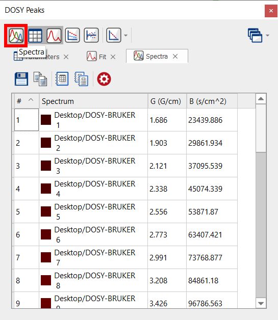
From that panel, you will be able to get information about each peak and the diffusion values from the fit analysis. Clicking on the 'Spectra' button will display information about each trace of the stacked plot:
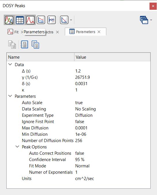
Selecting the Parameters button will display some useful information from the metadata:
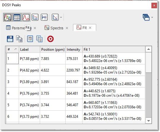
Selecting 'Fit' will display a table with information about the fitting values for each peak:
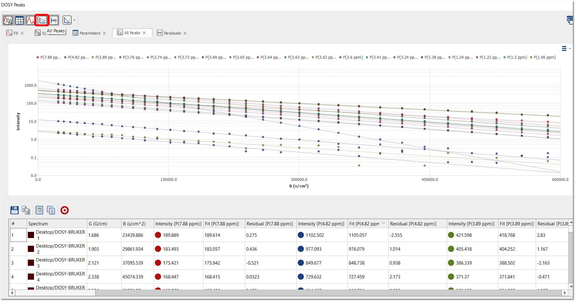
Click on 'All Peaks' button to display the Intensity/B graph of each peak of the applicable trace of the stacked plot:
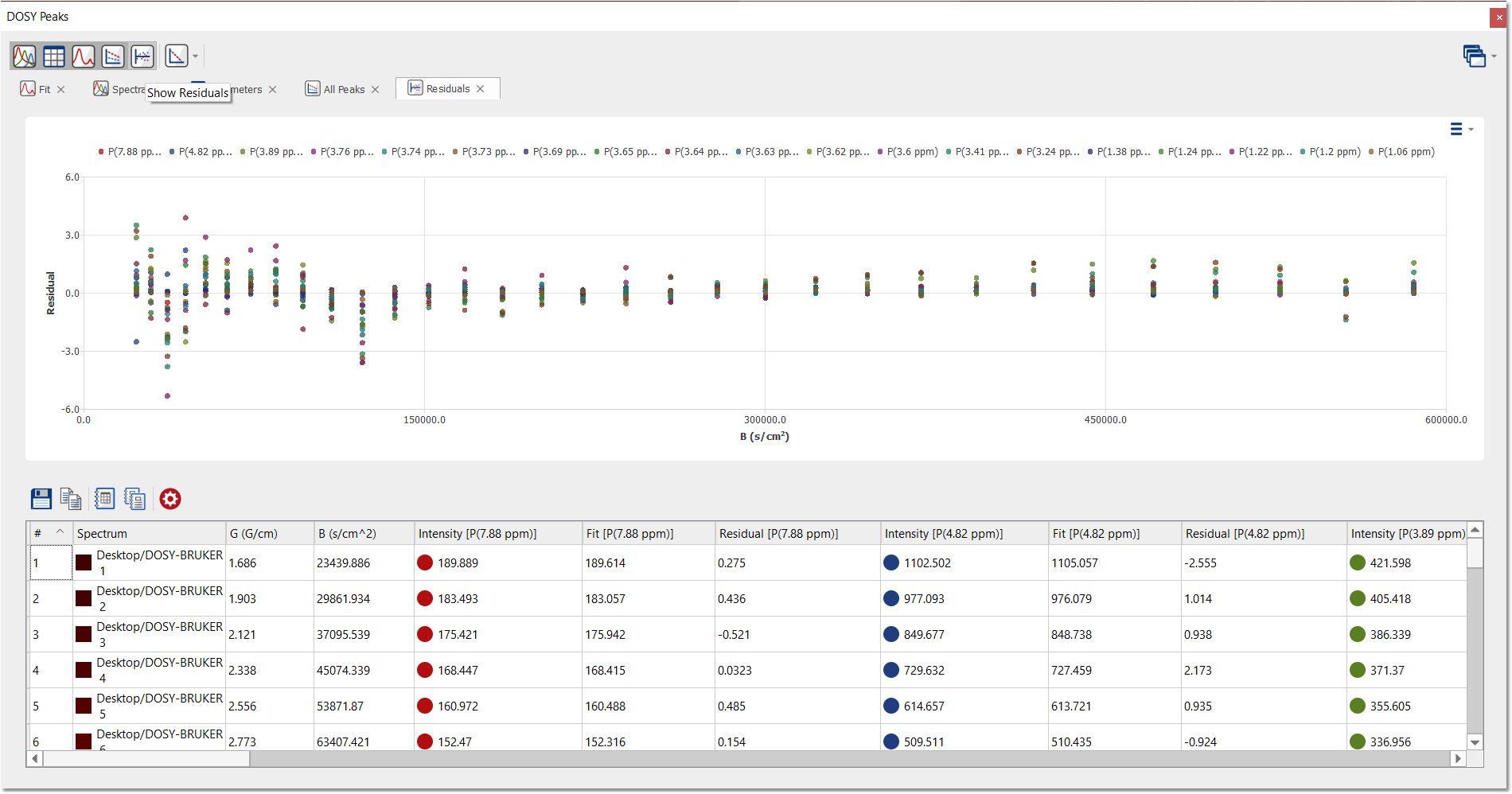
Click on the 'Show residuals' button to display the residuals of each fitting:
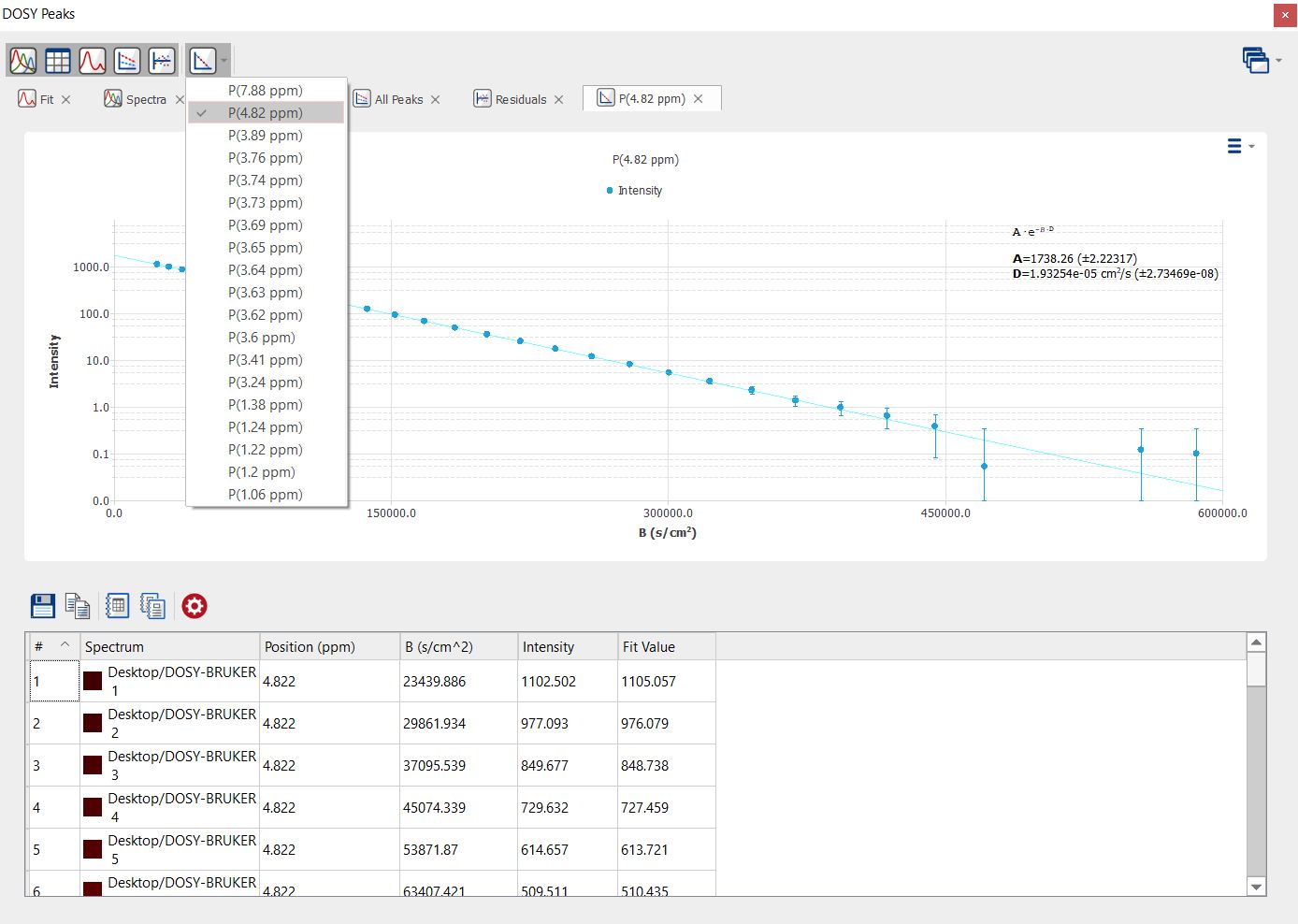
You can also select the individual fitting curves per each peak by selecting them from the scroll down menu:
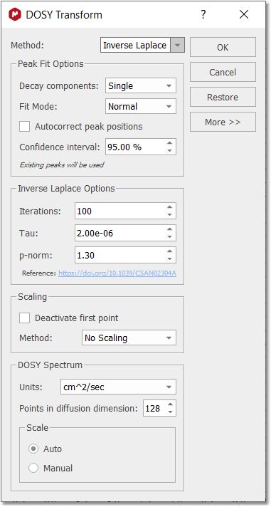
Inverse Laplace Method Inverse Laplace transform is a technique, which gives a continuous distribution of the diffusion coefficients/relaxation rates. It’s an alternative technique to Peak Fit which rather uses discrete number of components in the decay. Finding a distribution of decay constants from a data with discrete number of points, affected by experimental noise is an ill-defined mathematical problem which may have multiple solution, valid mathematically, but not necessarily meaningful in the chemical nature. A lot of efforts has been done to tackle the problem: usually some sort of regularization is used to restrict the distribution search. For example, the distribution is assumed to be “smooth”, has the minimal “entropy” or so on.
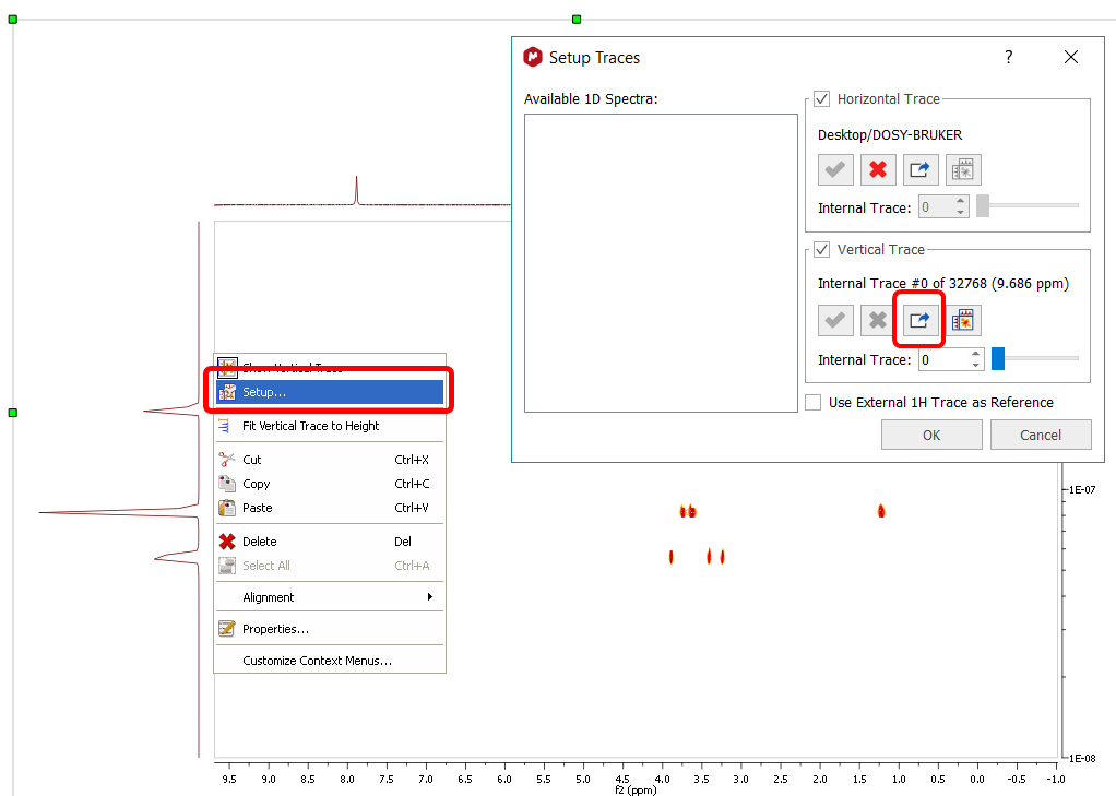
There is a number of options which affects the method performance and final results. They are available for user modification if Method: Inverse Laplace is selected. •Iterations: the number of iterations steps, used for iteratively re-weighted least-square algorithm. The number should be sufficiently large to solutions to converge. Default value is 100 but value around 20 should give solutions with reasonable quality. The computation time is roughly proportional to this parameter. •Tau: the ratio between root-mean-squared deviation and the regularization term in objective function used for optimization. Very small values of tau make the root-mean-squared deviation dominant, but the lack of regularization can cause instability of solutions and solutions with many unnaturally sharp peaks. Very large value can cause “over-smoothening” of the solution. See original paper and the supplementary materials for the examples how tau affects the results. •P-norm: coefficient p for lp-norm regularisation. The value is in the limits 1≤p≤2. Values of p>1 produces “smoothed” solutions. See the original paper for the discussion of lp-norm regularisation. The original paper proposes a method for automatic determination of the p value. However, the procedure is too time-consuming to be used for transforming to 2D map with many point in chemical shift dimension. Instead, the parameter p is adjustable by the user. Parallel CPU computation is used on supported platforms. The diffusion or relaxation scale can be represented either as logarithmic or as a linear one. The direction of values in the scale (ascending or descending) also can be changed. These changes are made for compatibility with external NMR software (e.g. Bruker TopSpin) as well as following preferences of several users. The features can be found in the More section of the DOSY/ROSY transform dialog. More information can be found here: https://doi.org/10.1039/C5AN02304A Bayesian DOSY and quantification The Bayesian DOSY-data transform algorithm (BDT) in Mnova is inherently linear so amplitudes of "responses" are proportional to "inputs". However, that is not the whole story: The Bayesian approach always involves a final normalization which is pretty much a matter of choice and in BDT leaves a lot of degrees of freedom to play with. We normalize each column in the resulting 2D map so that it matches the point in what would be the 1D spectrum corresponding to zero gradient. Such column normalization might look as involving a series of integrals along the D-axis, but it is not, because an "integral along the D-scale" makes no sense (at best it might be viewed as a kind of Stieltjes integral, with properly defined D-scale interval weights). It is a trick, an intuitive hack, which however greatly alleviates the quantitation problem. Ratios of peak integrals in the projection therefore come quite close to ratios between component quantities. However, given the inherent impossibility to justify an "integral along D or logD", we tend to avoid the concept, at least for the time being, especially should somebody integrate over very broad intervals of D's, or compare two integrals around very different D values. From this point of view, given the kind of normalization we have adopted, peak heights are more rigorous quantities - unless the peaks of a component get misaligned on the D axis because of artifacts (for that reason a moderate integration including just very few D-scale points might be acceptable). So, BDT will help you to obtain the relation of each compound by just integrating the diffusion trace. To do that, just right click on the trace and select 'Setup' in the contextual menu to display the 'Setup Traces' dialog box. Once there click on the 'blue arrow icon to extract the 'Vertical Trace'. Please make sure that this trace is the 'Internal Projection' (Sum):
This will extract the trace to a new page. Finally integrate the signals of this trace to get the applicable ratio of the compounds:
See this webinar for further information about DOSY processing. |