Integration


Integration |
|
|
Spectral integration can provide invaluable quantitative information about a molecule as the integral of a spectrum indicates the number of nuclei which contribute to a given line (or set of lines).
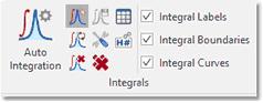
Mnova implements a series of integration algorithms for both 1D and 2D data sets. These algorithms can be accessed via the menu item 'Analysis/Integration':
Autodetect Integration
1D spectra
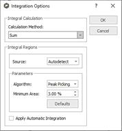
The program automatically determines the regions containing signals. The algorithm uses the following options:
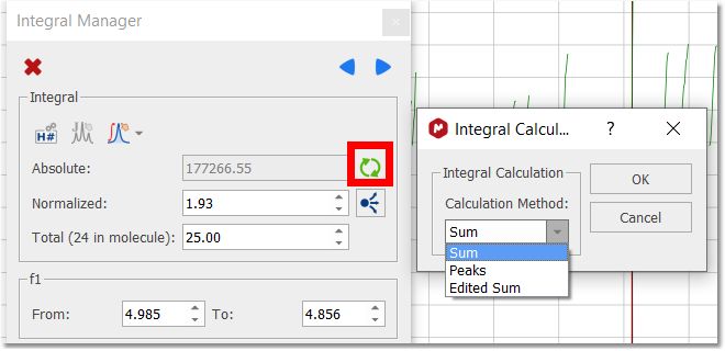
•Calculation Method: you can select between 'Sum' (classical integration, faster than 'Peaks' but without deconvolution), 'Edited Sum' or 'Peaks' (it takes into account only the integrals of the GSD spectrum and because of the deconvolution applied, it is slower than the 'Sum' algorithm). In the Peaks calculation method, you can select what peaks will be taken into account for the integration (for example, only compounds peaks and not solvent or impurity peaks, etc...)
Edited Sum: in this integration method, the values from Sum method are corrected using a correction factor:
Sum(Ps_i)/Sum(P_i): where "Ps_i" are the selected peaks (by default, including Compound peaks and excluding Hidden, C13_Sat and Rotational); "P_i" are all peaks in the integration range. Int (Edited Sum) = Int (Sum)* (Sum(Ps_i)/Sum(P_i))
For further information about the edited Sum algorithm, please check this paper: http://pubs.acs.org/doi/abs/10.1021/acs.analchem.5b04911
•Algorithm: you can select between the regular algorithm which is called 'Derivative' and the new algorithm based in the 'Peak Picking'.
- Derivative: you will find the options described below: Sensitivity: This value controls how small peaks can be detected. It is a kind of smoothing parameter so that large values will filter out noisy signals. Peaks of small intensity will also be discarded in the automatic integration. Reduce this value if some small signals of interest are not detected. Merging distance: This parameter is used to control the separation of integrals. Integral regions separated by less than this value will be merged into a single one
Minimum Area: Integrals with a value smaller than a given percentage of the largest integral will be discarded
- Peak Picking algorithm: this integral algorithm is based in the peak picking analysis. The user will be able to set the maximum value of the coupling constants (J Max), the Peak Width Factor and also the Minimum Area of an integral (integrals with a value smaller than a given percentage of the largest integral will be discarded).
Bear in mind that this algorithm is based on the peak picking results. If no peak picking has been applied, the program applies one on the fly automatically but the best way to proceed will be by first applying a peak picking to make sure that all the real peaks have been detected and, more importantly, artifacts and very small peaks (e.g. impurities) have not. So as always, it will be a good idea to apply a baseline correction, followed by peak picking – In this case, it’s important to ensure that the noise factor is right. Once you’re happy with the peak picking results, it’s time to apply integration algorithm. The critical parameter is the ‘peak width factor’; the larger this parameter, the wider will be the integral segments.
2D spectra Automatic integration of 2D spectra is based on the 2D peak picking algorithm. If no peak picking has been applied when the automatic integration command is issued, Mnova will automatically apply a 2D peak picking on the background and then, for every peak detected, it will find the applicable volumes. Thus, the options that control the 2D peak picking procedure also apply to the 2D automatic integration algorithm.
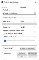
A series of Automatic Peak Picking Options can be controlled on the 'Peak Picking Options' dialog box, which can be accessed via the Peak Picking scroll menu (see the 'Peak Picking' section of this guide). The user can choose the noise factor (the higher the factor the less peaks will be picked), the peak type, whether to use parabolic interpolation, merging options for 2D multiplets, maximum number of peaks, etc. All these options can be evaluated interactively, so that their results can be viewed on screen in real time, by making sure the 'Interactive' box is selected.
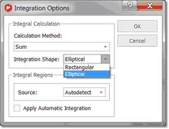
Peak volume integration in Mnova is measured as the sum of all digital intensities within the integration area (footprint). This footprint can be of 2 shapes: rectangular or ellipsoid footprints. In low resolution spectra with no significant fine structure, the ellipsoids footprints fit well, whereas higher resolution spectra tend to show rectangular patterns according to the projections of the correlated individual multiplets. The default setting is with ellipsoids. But you can change it to rectangular in the integration options.
By the way, you can also manually change the size of a footprint by click-and-drag on one of the edges of the footprint.
Predefined Regions Integration
The user will be able to predefine the integral ranges to automate the integral analysis. Just go through the following procedure:
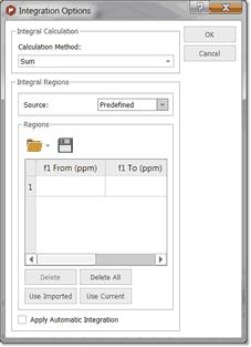
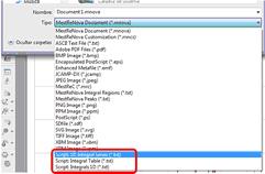
1. Open the 'Integral Option' dialog box (by clicking on 'Options' in the 'Integration' scroll down menu) and select the Method: 'Predefined Regions' as is shown in the picture below:
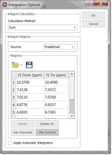
2. This will display a new dialog box, where the user will be able to select the desired ranges to apply the integration. If you have already integrated the spectrum you can click on the 'Use Current' button to import the integral ranges:
Clicking on OK, will apply the integrations to the current spectrum and keep the regions to apply further integrations to additional spectra by just clicking on 'Predefined Regions' in the Integral menu:
The user will be able to save these regions for later uses, by clicking on the 'Save Integral Regions' icon which will be loaded by clicking on the 'Load Integral Regions' icon. To save the integral regions, follow the menu 'File/Save as' and select 'MestReNova Integral Regions'.
You will also be able to use the original Bruker integrals by using the 'Use Imported' button. Please bear in mind that if you import a Bruker file with MNova, the integrals will appear automatically, however if you open and old Mnova-document with Bruker data then this button is the way to use Bruker ranges. With the 'Use Imported' button you will be able to reload the original Bruker integrals.
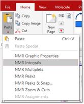
To copy&paste the spectral regions from one spectrum to another, just press 'Ctrl/Cmd+C' in the original spectrum and then follow the menu 'Home/Paste/NMR Integrals' in the other spectrum (or spectra, if you have previously selected them in the page navigator):
The integral list can also be exported as an ASCII file by following the menu 'File/Save as' and selecting 'Script: Integrals 1D (*.txt)' (or 2D depending on the dataset). You can also export the integral series and tables:
Manual Integration (shortcut: I)
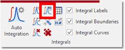
First, select integration mode by clicking on the Manual integration command as depicted below:
.
•Next, click and drag with the mouse to select the area to be integrated •The first integral will be normalized to 1.0. All following integrals will be referenced relative to the first integral.
Follow the menu 'File/Save as' and select 'MestReNova Integrals (*.txt)' to save the integrals list as a 'text file'
Integral Settings:
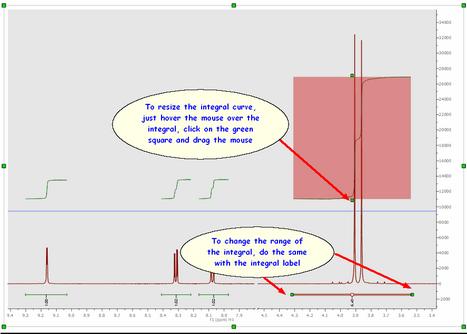
All the integral curves are mouse-sensitive and they respond to usual mouse operations. If you want to move up or down all the integrals, just click and drag (with the left mouse button) over anyone of the integrals (notice that hovering the mouse over the integral will highlight it in red). If you keep pressed the SHIFT key at the same time, the height of the integral curves will be changed.
The same effect will be obtained if you hover the mouse over integral curve, click on one of the green squares and drag the mouse up or down. If you want to change the range of the integral, do the same with the integral label (notice that once you hover the mouse over the green squares of the integral curve or label, the mouse pointer turns to vertical or horizontal arrows, respectively).
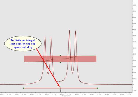
Cutting Integrals: to divide any integral just by clicking on the red square of the integral label and dragging the mouse:
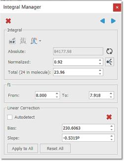
Integration Manager (shortcut: Shift+I): The integral editor will be displayed by double clicking on any integral curve. From there, you can change the integral range, normalize the integral to a specific integral, navigate through them and also to reference integrals to the total integral value for the spectrum.
You can manually add integrals and multiplets using different integration calculation methods (Sum, Edited Sum and Peaks). To avoid misunderstandings in the integration results, you can track the method used in each integral/multiplet. This will be displayed in the Integral/Multiplet Manager, where there is an option to recalculate each integral/multiplet with ability to choose the integration method in each case.
A similar option can be found under the Analysis/Integrals menu.
The user can resize the limits of the integral by using the arrow buttons
Bear in mind that you are able to navigate over the integrals by using the 'Previous or Next' icons.
If you want to resize the height of the integral curve, just hover the mouse over one of the integral curves and hold down SHIFT, click on left mouse button and drag up or down (to increase or decrease the height).
If you want to normalize the integrals, just overwrite the desired value on the 'Reference edit box' (on the Integrals Editor') and press OK, all integrals will update with reference to the chosen one. The user can also delete an integral one by one by clicking on the 'Delete' button.
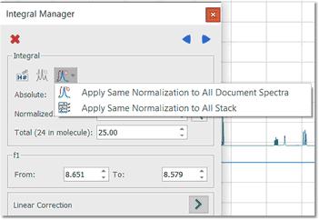
You can apply the same integral normalization to all the spectra (in the current document) or to all the traces of a stack plot by selecting the applicable option, as you can see below. This is very useful if you need for example to determine relaxation times from a series of 1D spectra, to be able to compare the integral values between the different traces.
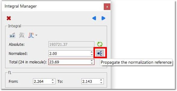
You can propagate the normalization reference of any signal to all the traces in a 1D or 2D stack by using this command:
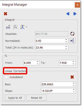
Linear Correction: Linear correction is basically a straight line built connecting the left and right boundaries of every integral in such a way that the final area will include only the integral above that line. In other words, if A is the total area under the peak(s) and B is the area under that straight line, the reported integral R will be: R = A – B Mnova has an option to automatically calculate this straight line. In order this to work properly, it’s recommended to have a good digital resolution (e.g. by applying ZF), as the program utilizes 3 points at both edges of the integral to build the straight line. If you want to apply an integral correction or rather, a linear baseline correction just on the integral region, just adjust the Bias and Slope parameters or check the Autodetect box:
Use the controls for Bias and Slope correction as follows:
- Adjust the Bias parameter until the initial (left) part of the integral is flat. - Adjust the Slope parameter to flatten the top (right) part of the integral curve.
The Auto box computes the Bias and Slope values automatically. The button Apply to All is used to correct all the integrals simultaneously.
We strongly recommend to correct the baseline prior integration using any of the baseline correction algorithms.
Likewise, if you press the right mouse button on an integral, you will get a pop-up menu with the following options:
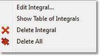
Edit Integral: displays the Integration Manager dialog box. Show Table of Integrals: to show the integrals table Delete Integral: deletes the current integral. Delete All: deletes all integrals. Autodetect Nuclides Count: this command will be very useful to count the nuclides present in any spectrum. Integration only gives information on the relative number of different nuclides. From a practical stand point, first the absolute integral values are computed and then the integrals are normalized (referenced).
For example, if we know that a given integral corresponds to a CH3 group, we can set it to a value of 3 so that all other integrals will be scaled accordingly. Note that these values are not exact integers and need to be rounded to the nearest integer to obtain the significant value. But that means that the reference should have correct intensity to start with, which is not guaranteed.
Our goal is to automate this process, that is, starting from the absolute integral values, automatically select the reference group and scale the remaining values in order to obtain the correct number of nuclides.
It is a simple algorithm to auto normalize the 1H NMR integrals without prior-knowledge. It will be useful especially for auto batch processing using the scripts of Mnova.
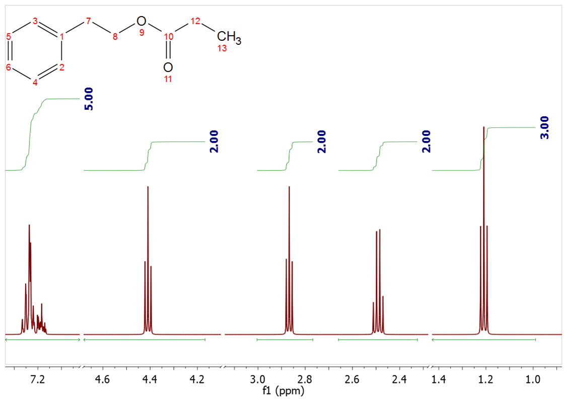
Starting from this situation:
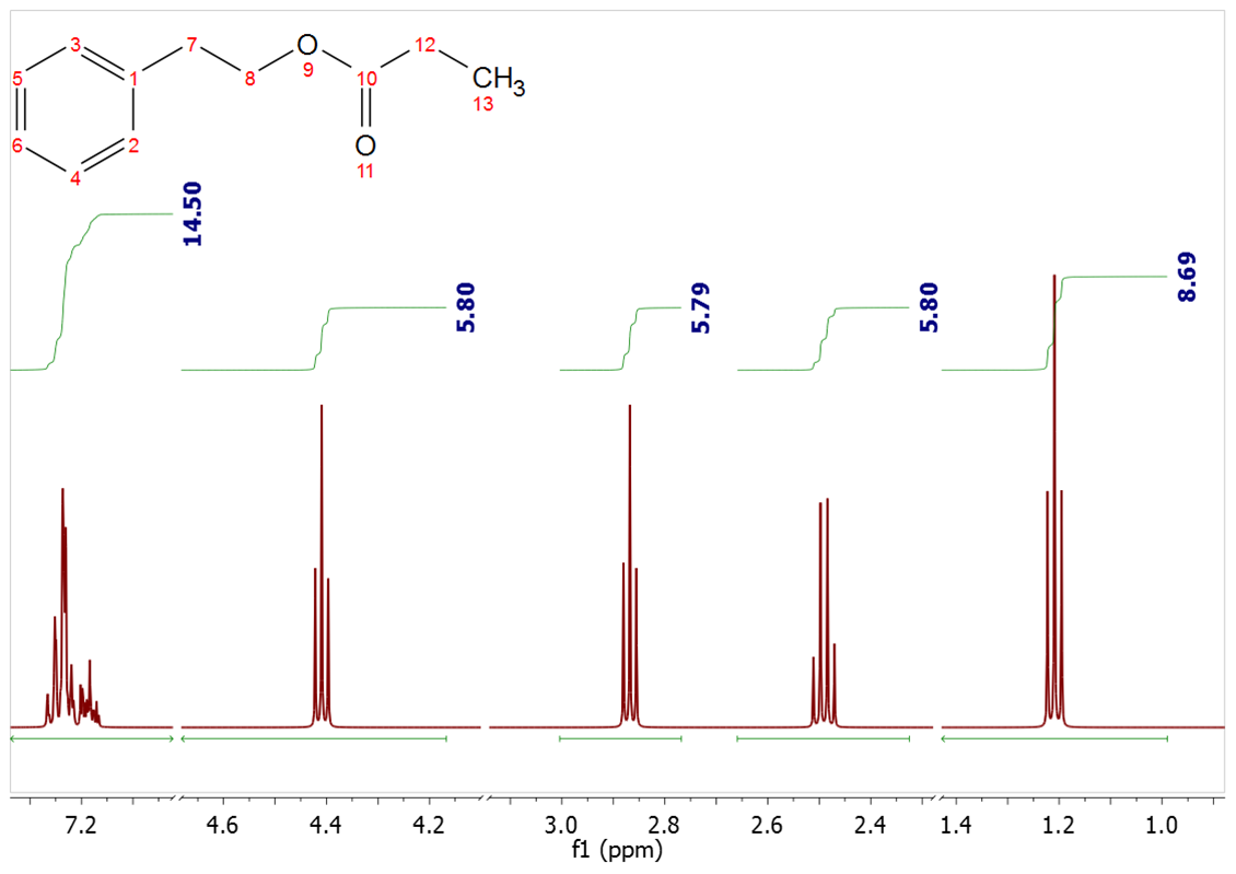
We can arrive to this one after having applied the algorithm:
See also: |