Covariance NMR

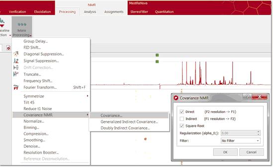
(Not available in Mnova Lite)

Resolution and sensitivity are two key factors in NMR spectroscopy. In the case of 2D NMR, the resolution of direct dimension (f2)  depends, among other things, on the number of acquired complex points whilst the resolution of the indirect dimension (f1) is directly proportional to the number of increments (or number of acquired FIDs). In general, it could be said that the resolution along the direct dimension comes for free in a sense that increasing the number of data points does not augment the acquisition time of the experiment significantly. However, increasing the number of t1 data points (increments) has a direct impact in the length of the experiment as can be seen from the Total acquisition time for a 2D NMR spectrum:

T = n*N1*Tav

Where n is the number of scans per t1 increment, N1 is the number of T1 increments and Tav is the average length of one scan. This usually means the resolution of the indirect dimension f1 is kept lower than that of f2.

You can easily apply the Covariance NMR tool just by following the menu 'Processing/More Processing/Covariance NMR/Covariance'. This will display the 'Covariance NMR' dialog box which will allows you to select the 'Regularization Factor', the 'Filter' and an 'Indirect Covariance NMR'. For further information about the CoNMR options, please check this paper: JBiomolNMR (2007) 38, 73–77

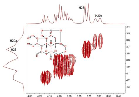
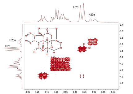
For example, let’s consider the COSY spectrum (magnitude mode) of Strychnine which has been acquired with 1024 data points in the direct dimension and with 128 t1 increments. It’s clearly appreciated that the resolution along F2 is much higher than the one along F1.

You can easily see that doublets corresponding to protons H20a and H23 are resolved in F2 but not in F1.

How could this be improved? We could try to extrapolate the FID (somehow) along the columns (F1) to a higher number of points (e.g. 1024). A well known technique is simply to add zeros, a process called zero-filling which basically is equivalent to a kind of interpolation in the frequency domain. For example, in this particular case we could try to extrapolate the FID along t1) from 128 to 1024 points in order to match the number of points along f2. The figure below shows the results:

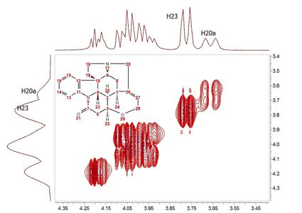
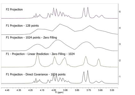
It can be observed now that the resolution along f1 is slightly higher than in the previous case but we cannot still appreciate the inner structure of the multiplets (e.g. H20a and H23). Zero Filling is certainly a good technique to improve resolution but of course, it cannot invent new information from where it does not exist. In this case we have zero filled from 128 to 1024 data points (e.g. 4 fold). In theory, zero filling by at least a factor of two is highly recommended because it enforces causality but beyond that, the gain in resolution is purely cosmetic. We might get more data point per hertz, but no new information is achieved as it’s shown in the figure above.

Is there a better way to extrapolate the FID? Yes, and the answer is very evident: Linear Prediction. In few words, Forward Linear Prediction uses the information contained in the acquired FID to predict new data points so that we are artificially extending the FID in a more natural way than with Zero Filling. Of course, we cannot create new information with this process but the resulting spectrum will look better. This is illustrated in the next figure:

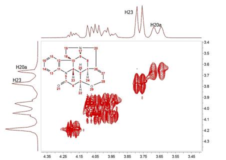
In this case, we have extended the t1-FID from 128 to 512 data points and then zero-filled up to 1024. Now we can see that the f1-lines are narrower but the couplings cannot be resolved yet.

In recent years there has been a great interest in the development of new methods for the time-efficient and processing of 2D (nD in general) NMR data. One of the more exciting methods is the so-called Covariance NMR, a technique developed by Brüschweiler et al. In fact, there are several types of Covariance NMR: Direct, Indirect Covariance NMR (there is a third method, Unsymmetrical Indirect Covariance which can be considered as a subtype of Indirect Covariance NMR). In this manual we will cover only the first type, Direct Covariance NMR leaving the other 2 types for future tutorials.

Before going any further with Covariance NMR, let’s see the results of applying this technique to the same spectrum. This is what we get:

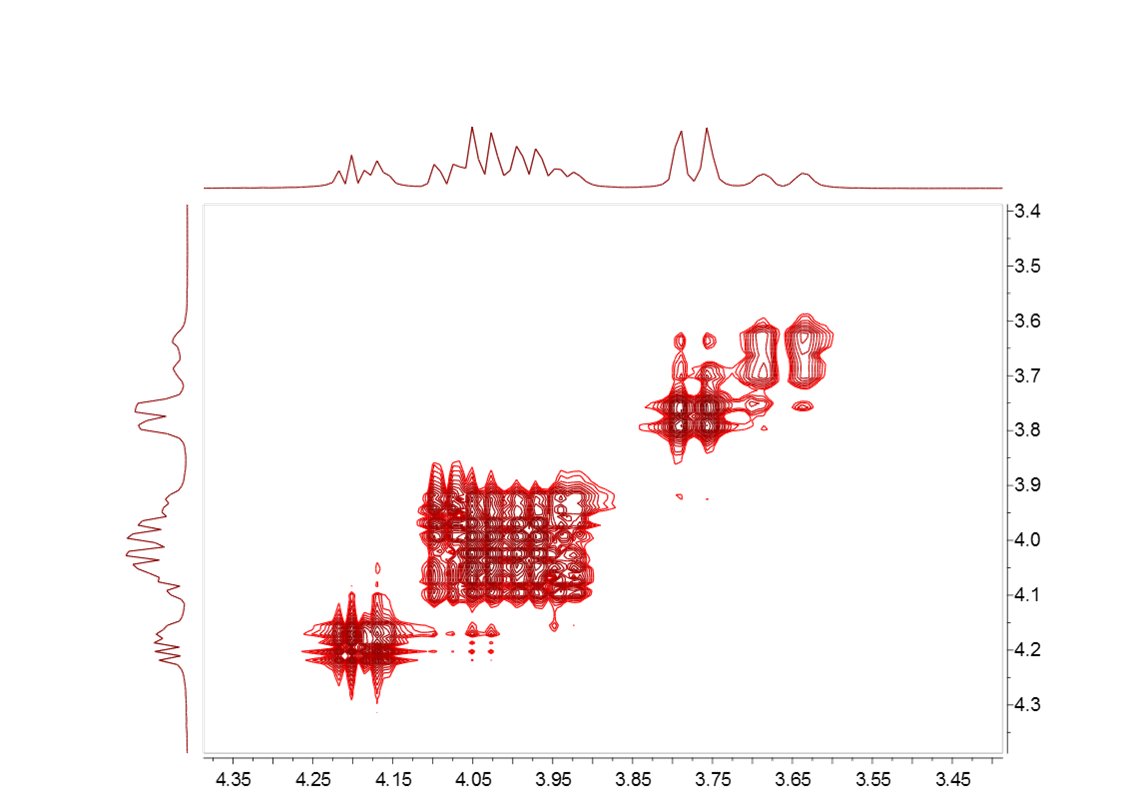
At first glance, this result looks like a kind of magic: Now the splitting of H20a and H23 are clearly resolved in both dimensions. Actually, the resolution along F1 is virtually analogous to that of the F2 dimension.

How did we arrive to such a good result? From an intuitive stand point, what we have attained here was a transfer of the resolution of F2 to the F1 dimension. In other words, we have applied a mathematical process which takes advantage of the higher spectral resolution in the F2 dimension to transfer it to the F1 one.

Mathematically, direct Covariance NMR is extremely straightforward as defined by the following equation:

C = (FTF)        (1)

Where C is the symmetric covariance matrix, F is the real part of the regular 2D FT spectrum and FT its transpose (NOTE: direct covariance NMR can also be applied in the mixed frequency-time domain, that’s, when the spectrum has been transformed along F2. In this case, a second FT will not be required – neither apodization or phase correction along the indirect dimension).

In order to approximate the intensities of the covariance spectrum to those of the idealized 2D FT spectrum, the square root of C should be taken. Root squaring may also suppress false correlations that many be present in FTF due to resonance overlaps. Taking the square root of C matrix is in practice done using standard linear algebra methods (in short, diagonalizing the matrix and then reconstruct C1/2 using eigenvectors and square root of eigenvalues).

So direct Covariance NMR is able to produce a 2D spectrum in which the resolution in both dimensions is determined by that resolution of the spectrum in the direct dimension.

Let´s see a stacked plot representation with the 1D projections obtained from the different processing methods described here (Zero-Filling, Linear Prediction and Direct Covariance NMR). You can see in the picture below the power of the Covariance NMR method.  

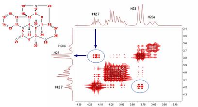
Covariance NMR spectroscopy provides maximal resolution along the indirect dimension, but when the number of acquired data points is too small, the covariances exhibit poor statistics that manifest themselves as spurious cross-peaks. For example, in this case we can see some unexpected cross peaks (e.g correlation H27 and H23 which in principle should not appear in a GCOSY spectrum, but rather in a TOCSY spectrum). Some other artifacts might also arise when protons of different spin systems are coupled to resonances with overlapping proton multiplets.

Mnova includes a novel filter which addresses this situation. This filter combines the standard 2D FFT spectrum with the CoNMR version in such a way that the resulting spectrum, while keeping the high spectral resolution along F1, it’s free of artefacts:

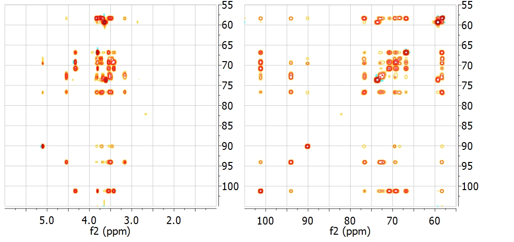
INDIRECT COVARIANCE NMR

Interestingly, if we have a heteronuclear spectrum, we can transfer the correlation information from the indirect dimension to the direct one by simply changing the order in which the multiplication is carried out:
 
Cindirect = (F·FT) 1/2
 

For example, the spectrum below shows the HSQC-TOCSY spectrum of sucrose (left) and its resulting indirect covariance counterpart (right) which contains essentially the same spin-connectivity information as a 13C-13C TOCSY with direct 13C detection:
 

 
The advantage is obvious: Indirect Covariance NMR yields a 13C-13C TOCSY correlation without having to detect the 13C nucleus. In other words, it brings in a sensitivity increase of 8 over a 13C detected experiment. Of course, in indirect covariance NMR spectroscopy, the spectral resolution along both frequency axes is determined by the sampling along the evolution t1 time.

UNSYMMETRICAL COVARIANCE NMR

You can also carry out unsymmetrical Covariance NMR with Mnova. However, as opposed to direct/indirect covariance NMR where one needs to deal with just one single spectrum, unsymmetrical NMR processing is probably not as intuitive as it's necessary to use 2 independent spectra and we have decided to implement it using a very open and flexible approach, that is, by using the spectral arithmetic module.

There two ways to apply an 'Unsymmetrical CoNMR' with Mnova:

1. Using the Arithmetic feature

2. Using the Generalized Indirect Covariance NMR

As you can see above, Covariance NMR is all about matrices operations. When you use direct/indirect CoNMR you simply multiply the spectrum matrix by its transpose where the order of the multiplication depends upon the CoNMR technique (direct vs indirect). The same concept applies to unsymmetrical CoNMR where you just need to multiply one spectrum by the transpose of another one.

Let´s see an example to apply an unsymmetrical CoNMR by using the 'Arithmetic' feature of Mnova, assuming that matrix A corresponds to an HSQC spectrum and matrix B corresponds to a COSY (or TOCSY) spectrum, unsymmetrical CoNMR can be achieved by the following matrix operation:

C = A * TRANS(B)

Where TRANS denotes matrix transposition.

It's important to bear in mind that with any algebraic matrix operation, it's necessary that matrices A & B are compatible according to their row/column dimensions.

To carry out unsymmetrical CoNMR, just open the 2 individual spectra in Mnova, process then as usual (making sure that the sizes are compatible) and finally go to Processing/Arithmetic to enter the desire equation (e.g. A * TRANS(B) )

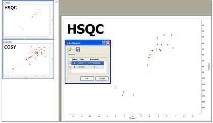
Let´s see step by step, how to generate a HSQC-COSY from separate HSQC and COSY spectra with Mnova

1. Import the HSQC and COSY spectra into Mnova

2. Select both spectra in the page navigator and follow the menu 'Analysis/More Tools/Arithmetic'

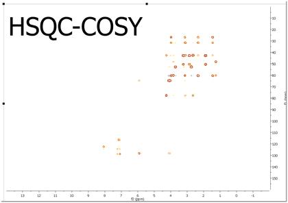
Finally enter the equation as depicted above "A*TRANS(B)".In this case A corresponds with the HSQC spectrum whereas B is the COSY experiment. TRANS means the transpose operation.  

Once the operation has been applied, click on the fit to highest intensity button . You should get something like this:

Generalized Indirect Covariance NMR (GIC)

Multidimensional nuclear magnetic resonance (NMR) experiments measure spin-spin correlations,which provide important information about bond connectivities and molecular structure. However, direct observation of certain kinds of correlations can be every time-consuming due to limitations in sensitivity and resolution.

Covariance NMR derives correlations between spins via the calculation of a symmetric covariance matrix, from which a matrix-square root produces a spectrum with enhanced resolution. The covariance concept has also been adopted to the reconstruction of non symmetric spectra from pairs of 2D spectra that have a frequency dimension in common. Since the unsymmetric covariance NMR procedure lacks the matrix square root step, it does not suppress relay effects and thereby may generate false positive signals due to chemical shift degeneracy. This generalized covariance formalism permits the construction of unsymmetric covariance NMR spectra subjected to arbitrary matrix functions, such as the square root, with improved spectral properties.

This method is basically the same as the above one (Arithmetic) but using a more rigorous mathematic formalism which allows to minimize the number of false positive peaks, because now the user will be able to do the square of the two matrix product (or any other values of the lambda parameter; ie: 0.25)

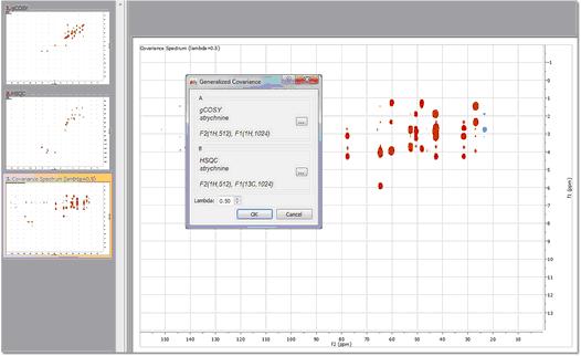
To use this method, just load your datasets and follow the menu 'Processing/More Processing/Covariance NMR/Generalized Indirect Covariance'. Finally select the spectra that you want to use and enter the value for the lambda parameter.

Please bear in mind that both spectra must have the same number of points in F2 to apply GIC

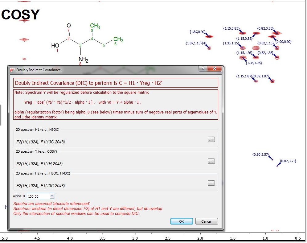
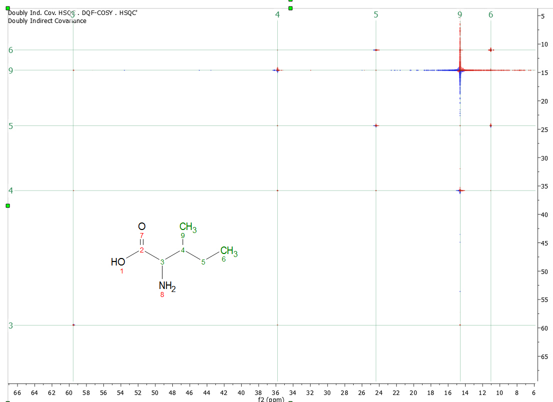
Doubly Covariance NMR

The Double Covariance NMR spectroscopy, is extremely useful for structure elucidation as resulting spectrum is actually a carbon-connectivity map that can be directly analyzed with basic graph theory to obtain the skeletal structure of a molecule or even of individual mixture components or their fragments.

In the example shown below, we have a COSY and a HSQC loaded in the the same document.

After having followed the menu 'Processing/More Processing/Covariance NMR/Doubly Indirect Covariance', we will get a synthetic spectrum (HSQC,HMBC) with the carbon-connectivity map:

For further information about CoNMR, please read our blog:

http://nmr-analysis.blogspot.com/2008/10/introduction-to-covariance-nmr.html

http://nmr-analysis.blogspot.com/2008/11/indirect-covariance-nmr-fast-square.html

http://nmr-analysis.blogspot.com/2008/11/removal-of-artifacts-in-direct.html

An this review: http://www.ebyte.it/library/docs/nmr14/2014_NMR_Cobas_Covariance.pdf

and this paper: JBiomolNMR (2007) 38, 73–77

For further information about Doubly Indirect CoNMR: J.Am.Chem.Soc. 2010, 132,16922