Chemometrics - PCA

Principal Component Analysis (PCA) is a procedure which uses orthogonal transformation to convert a set of observations from correlated variables into a set of values of linearly uncorrelated variables (named principal components).

You can use Mnova for your PCA studies if you have a license for the Chemometrics plugin.

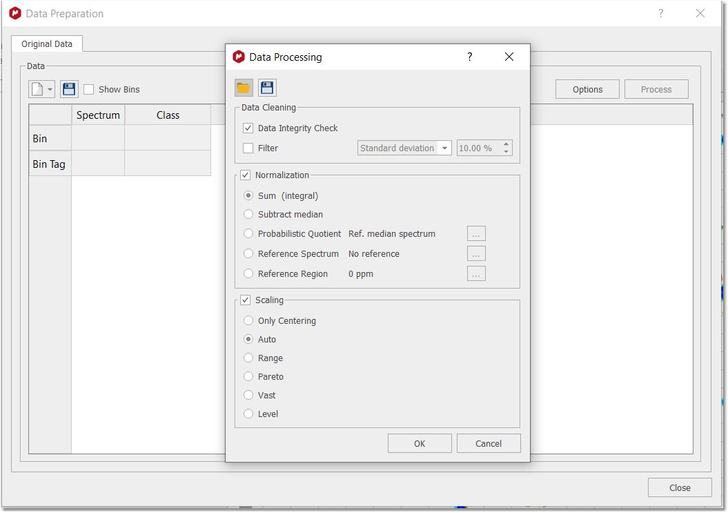
You will only need to load your 1D or 2D stacked spectra and follow the menu 'Chemometrics/Data Preparation. Clicking on the options button will display the 'Data Preparation' dialog box:

PCA1_0

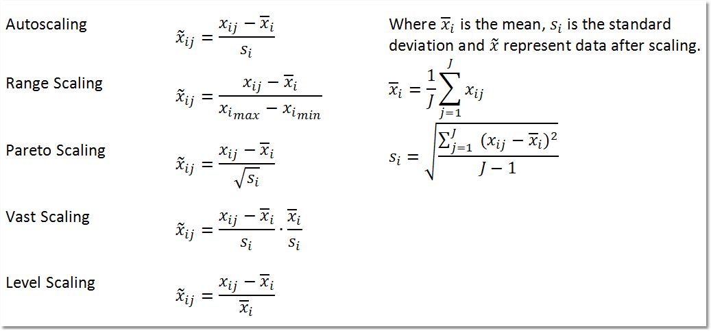
Data Cleaning: two options are available which could be used simultaneously.

a.Data Integrity Check replaces negative bin values (negative integrals) with zeros.

b.Filter. Filtering methods are used to remove bins that are null and do not displays any changes among spectra series. By default if a variable (bin) shows zeros among all rows (spectra) it is discarded. Five options are possible. In the first three options Standard Deviation, MAD and IQR a fixed fraction (default 10%) of the bins is discarded (e.g. if the matrix is composed by 100 bins it means that 10 bins are discarded, and the selection is based on the Filter method chosen). In practice Standard Deviation, Median Absolute Deviation and Interquartile Range are calculated for all bins. Furthermore an amount of bins (with the lowest SD, or MAD or IQR values) are discarded with respect a percentage value of the total bins.

In the case of Mean Value or Median Value, user is asked to input a value for the Mean or the Median. By doing, so only bins that display a lower value of the inputted one are discarded.

Normalization: it is an operation that is performed on the rows of the matrix. Four possible strategies could be selected:

c.Sum: every element on a row is divided by the sum of all elements of the same row;

d.Subtract Median: every element on a row is reduced by the median value of all the bins that constitute the same row;

e.Probabilistic Quotient: Normalization method proposed by Hans Senn et al.. For further information, please check this paper: Anal. Chem. 2006, 78, 4281-4290

f.Reference Spectrum (or reference series of spectra): upon normalization by the sum, every element of a row is divided by the corresponding element of the row of the selected reference spectrum (e.g. when you have a reference spectrum and you wish to compare all the other spectra relative to it). If you select a bundle of spectra (like all spectra belonging to the same class) normalization is performed on the calculated average spectrum.

g.Reference region (or bin): user inputs chemical shift value or range (in ppm) of a reference peak of interest and automatically MNova identify the bin(s) that comprises the selected peak/region. Furthermore every components of a row are divided by the reference component of the corresponding row.

Scaling: it is an operation that is performed on the columns of the matrix. Five different methods are implemented: Autoscaling, Range, Pareto, Vast and Level scaling. Mathematical operations applied are the follows:

scaling

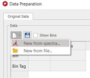
For further information about the different scaling methods, please visit this link.

The next step would be to select 'New from from spectrum' (or 'new from file' if you have any saved 'preparation file' from other experiment):

PCA_1-2

Check the 'Show bins' box to display the bins in the stacked plot.

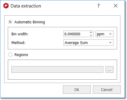
A new dialog will appear to select the binning options:

PCA_binning

If you are working with a 2D stacked dataset, you will get this dialog box:

2D_PCA

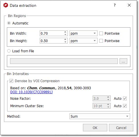
You can calculate the bin regions automatically or by loading a text file:

•Automatic: it creates the bin regions using a fixed bin size. You can set the bin width or bin height to Pointwise to work with the spectrum resolution in that dimension.

•Load from File: imports the bin regions from any existing 'MestReNova Integral Regions file' (which you can obtain from any integrated spectrum and following the menu "File/Save As/MestReNova Integral Regions (*.txt)")

From here, you can perform a VOI (Variable Of Interest) Compression, to reduce the number of interesting bins. It is recommended to do it for the binning methods: Sum, Average Sum, and Centered.

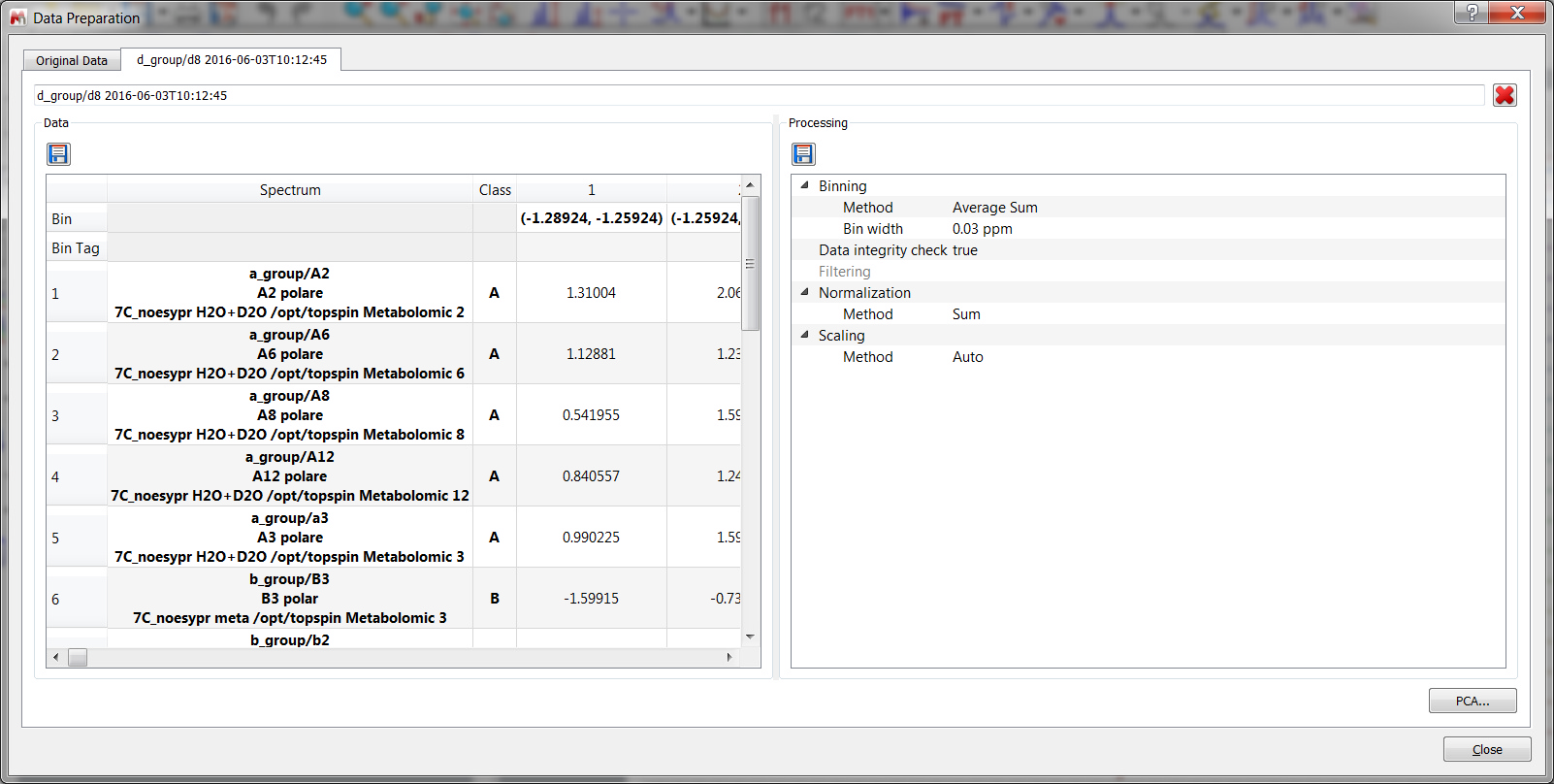
There are four binning methods are available: Sum, Average Sum, Center and Peak. The 'Sum' method will sum all the points of a bucket, the 'Average Sum' will divide the sum by the number of points in the bin, the 'Center' method will only return the value found in the middle of the bin. For example if a bin has 5 points it will return the value for 3rd point. The 'Peaks' method will perform firstly the GSD (Global Spectral Deconvolution) and then will apply binning over the peak table. For large dataset (more than 50 stacked spectra, it advisable to perform GSD before executing PCA module).

After having clicked on 'Process' button, you will get a new dialog summarizing the processing and allowing you to save the 'Data preparation file' or the 'Processing' file to be used in the future:

PCA_dialog

Finally, click on the 'PCA button' to select proportion of Variation (number of principal components) and to change the title:

PCA_panel

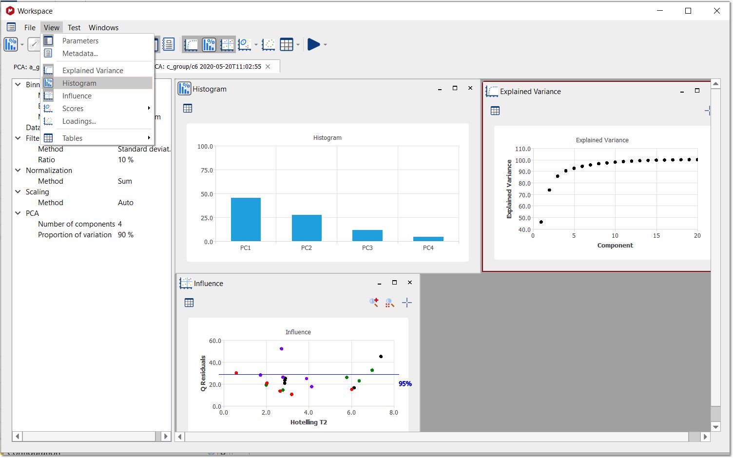
After having clicked on the 'OK' button; the Workspace panel' will be displayed. From the View menu, you will be allowed to display the 'Explained Variance', 'Histogram' and 'Influence' graphs. Right clicking (or Ctrl/Cmd+C) on any of the plots, will allow you to copy to clipboard, report or save the image:

PCA_2

Clicking on the 'Show Table' button, will hide/display the applicable table with the relative weight for each component:

show_PCA

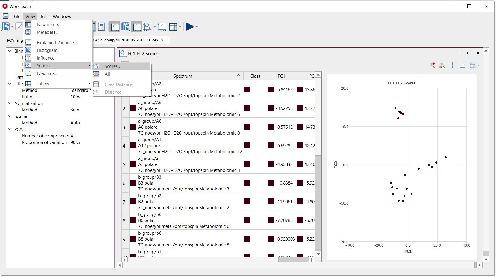
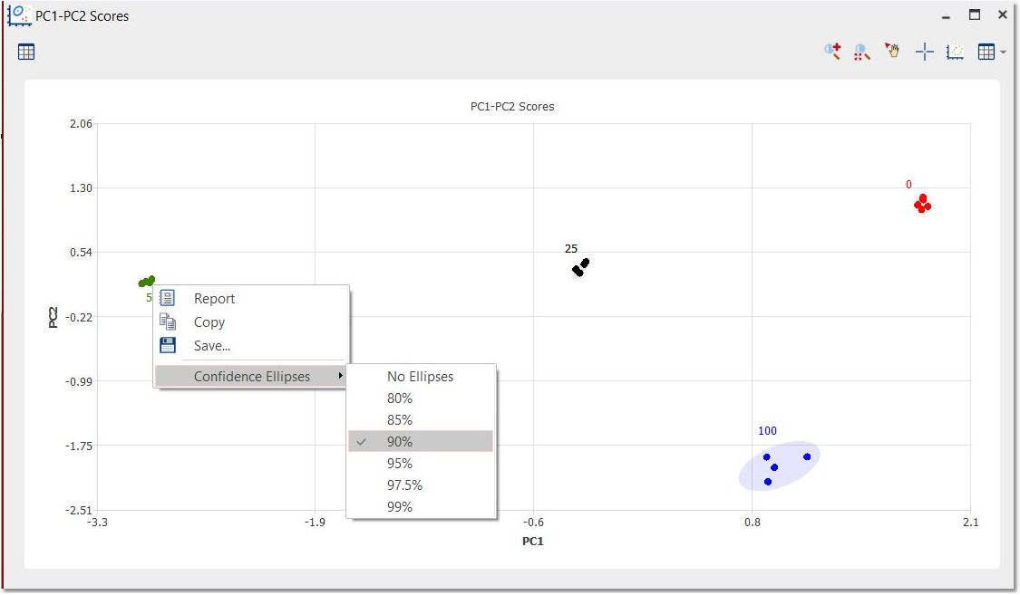
Selecting the 'Score Plot' tab from the "View/Scores" menu, will display a window like this:

PCA_4

You can display the confidence ellipses by right clicking and selecting the desired confidence value:

ellipes

For further information about how we are obtaining this value, please visit this link.

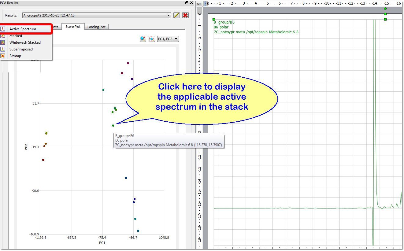
Each point of the 'Score Plot' is associated to a trace of the stack. If you are in the 'Active Spectrum' mode, you will get displayed the applicable spectrum when clicking on the point (of the Score Plot):

PCA_5

You can 'zoom in', 'reset zoom', use the crosshair or display the loadings plots by using the applicable buttons.

PCA_6

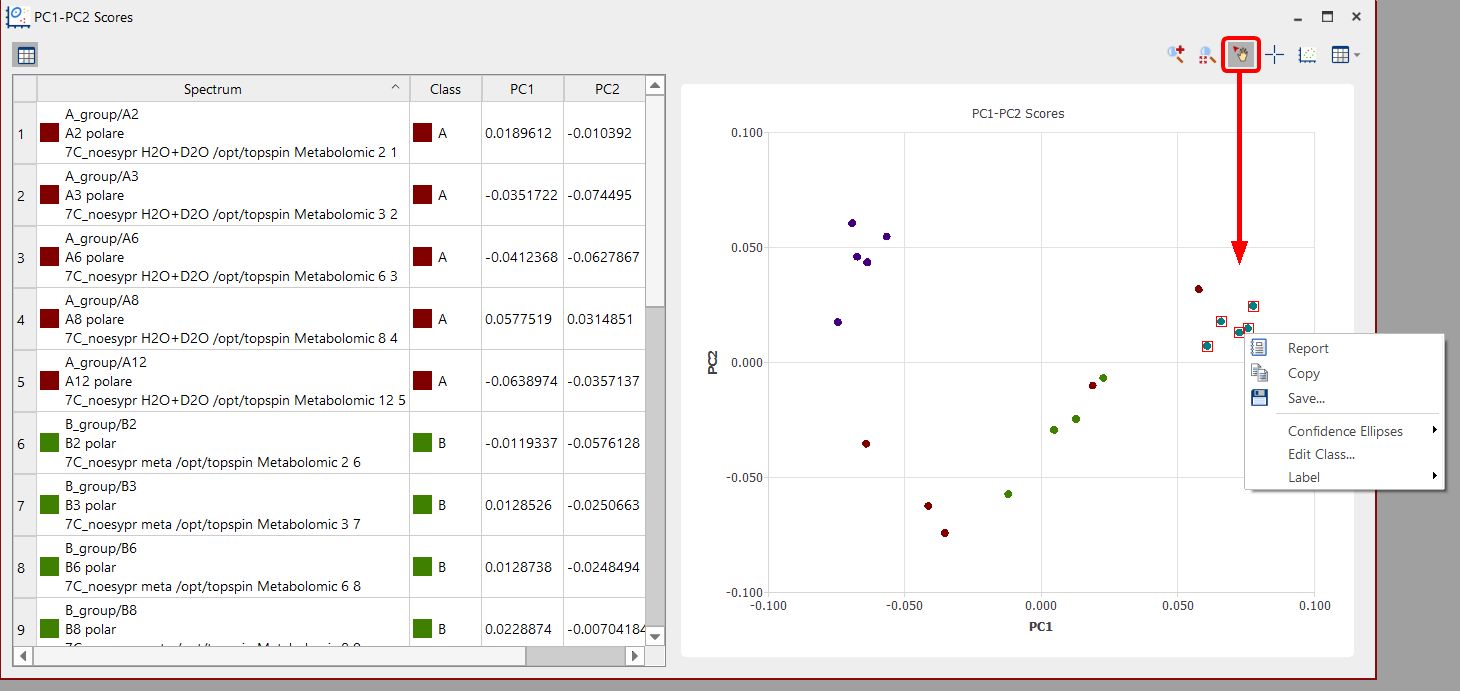
Clicking on the 'Show Table' button will display the results panel. From here you can select several rows and change the class or the color by right clicking on them (you can also change the class from the 'Stacked Items Table'):

class_PCA

You can also click on the 'Select points' button, hold down the shift key to click on the points of interest and right click on the them to select the confidence elipses, edit the class or show the label:

select_points

It will be possible to show the Spectrum Number in that label, but for that, it would be necessary to configure the title of the spectra in the stack (from the Properties dialog box) so that Spec Number is displayed in the first line:

label_PCA

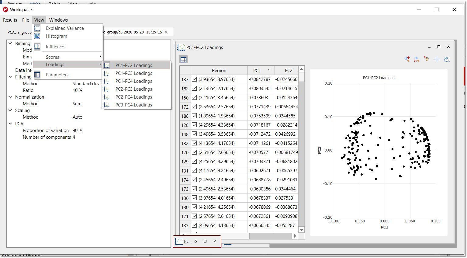
Select the applicable 'Loading Plot' from the View menu or by clicking on the applicable button of the Scores panel:

PCA_7

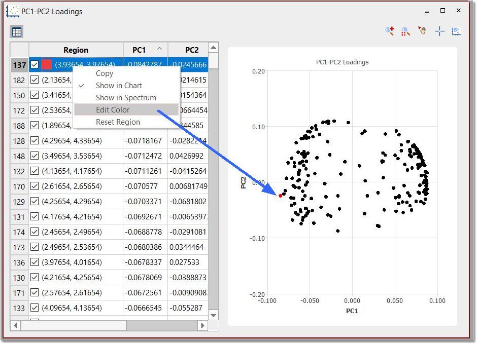
In this plot, each point will be associated to each region of the stacked spectra. You can change the visibility and colors of the bins by right clicking on the applicable row:

PCA_bin

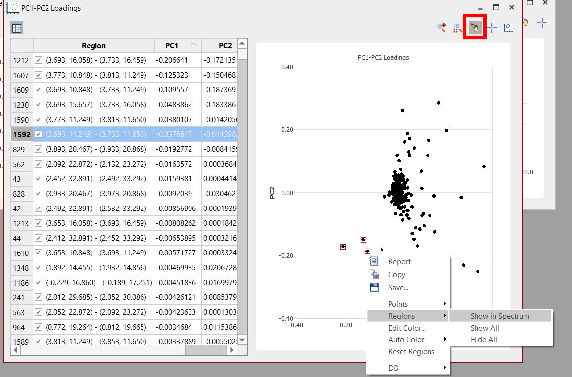
Using the feature to 'select points' in the loading plot and right clicking on them, will allow you to show the regions in spectrum or edit their color. Select 'Reset Regions' to get all of them in black.

select_point_loading

From the context menu, you can export the result as an image (png, svg, jpg or bmp) by clicking on the 'Save' option.

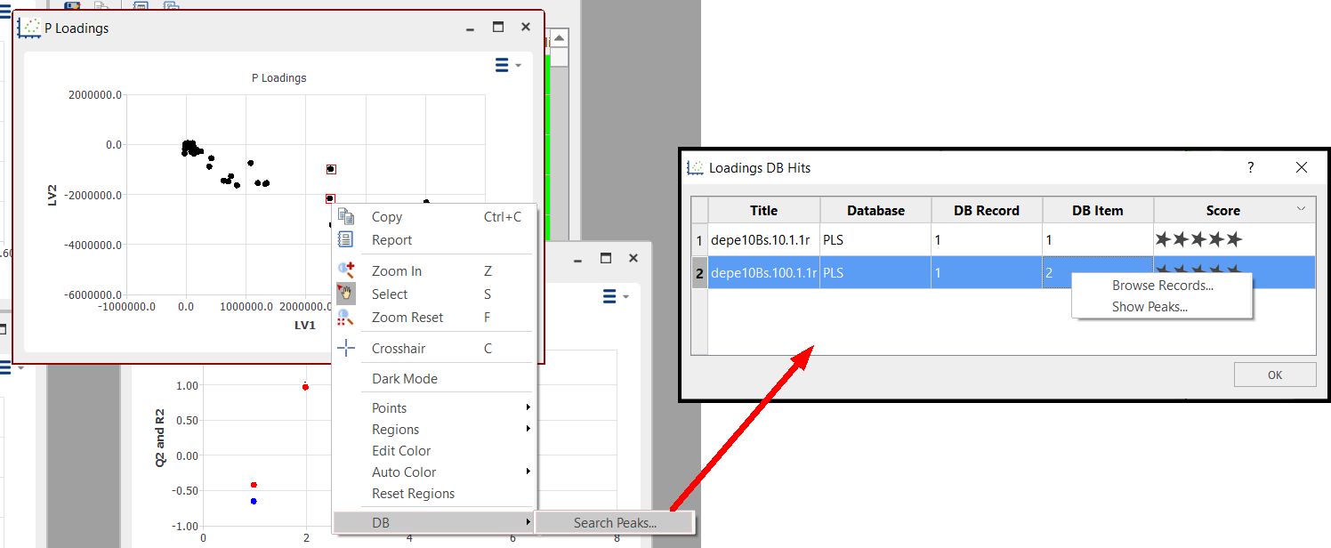
Click on the DB scroll menu to search for the Peaks in the Database:

clip0032

Double click on a row to display the record in the DB browser. Several records from several rows can be displayed by selecting the rows, right-clicking and selecting "Browse Records".

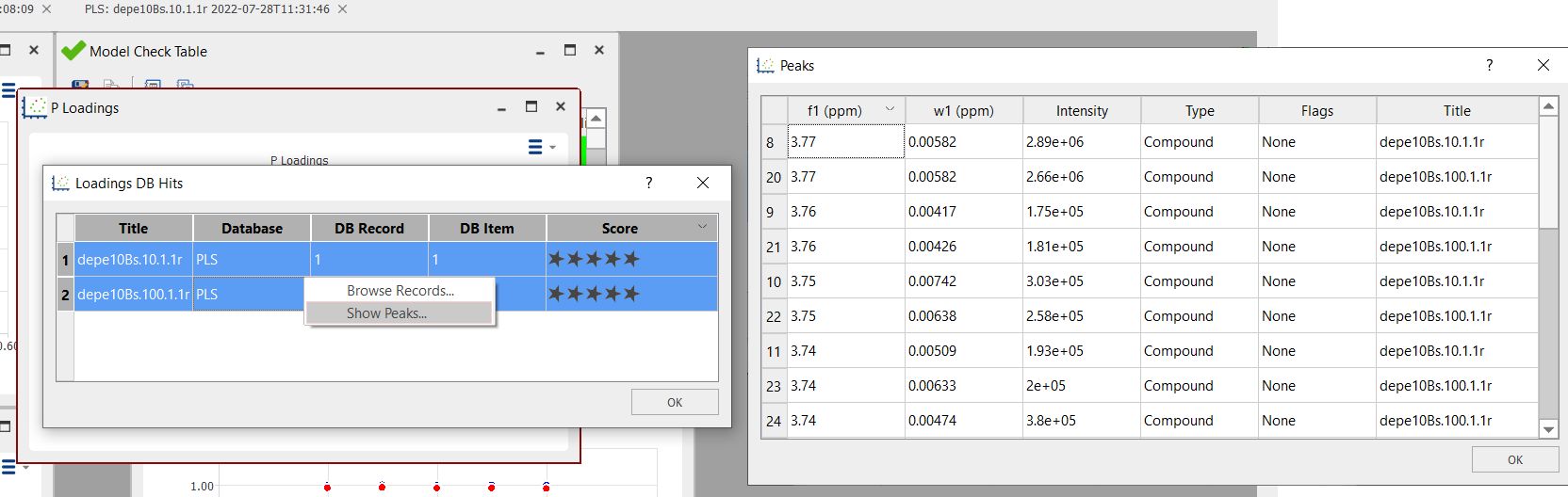
You can also display the list of found peaks by right-clicking and selecting 'Show Peaks':

found_peaks

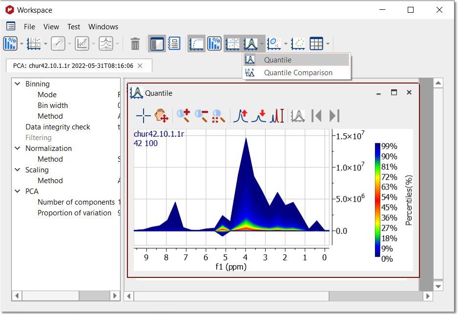
After having run the PCA, you can get the Quantile plot just by clicking on the applicable button:

quantile

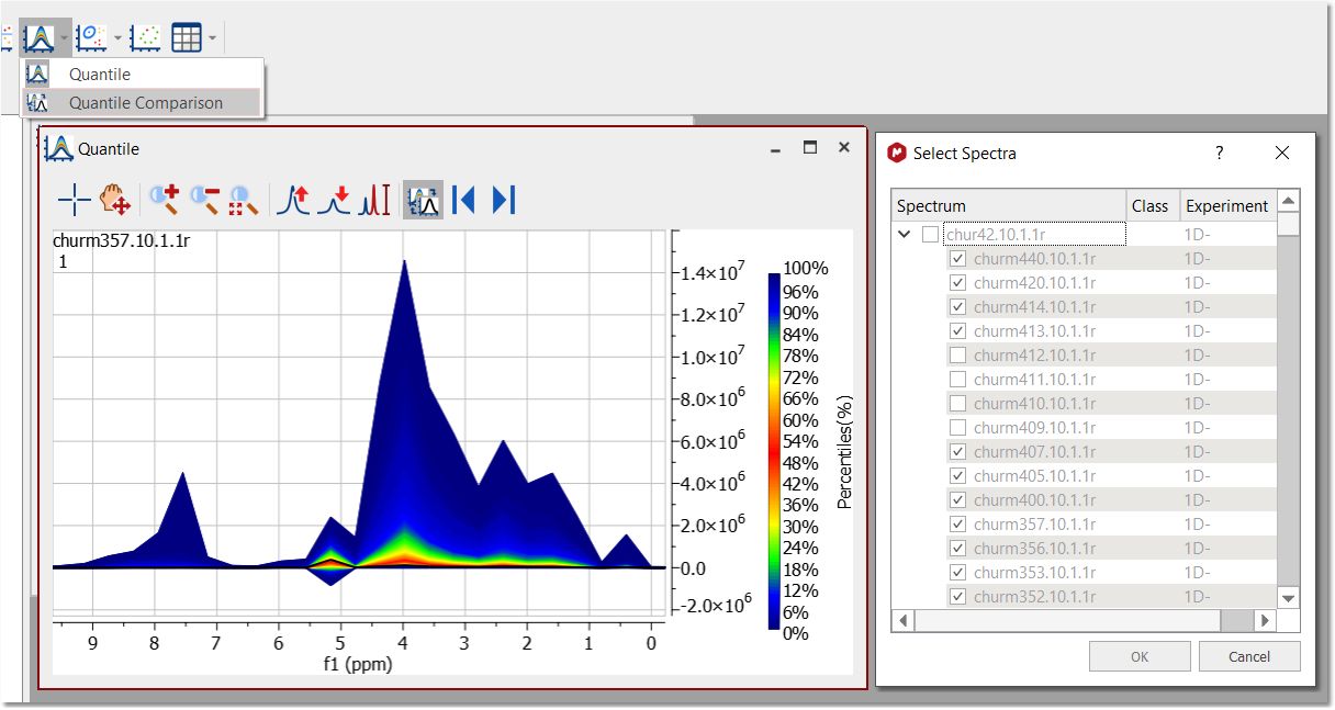
Quantile Comparison is available under Quantile scroll down menu. From here, you can select some/all the spectra in the stack to be overlaid one by one in the Quantile plot.

quantile2

If there are one or more spectra in the same document but not included in the stack, they can be also selected to be compared in the Quantile plot. Each overlaid spectrum shows in black color.

Ìn the toolbar of the Quantile plot there are specific buttons for the comparison:

1. Button to toggle between Quantile and Quantile Comparison.

2. Previous/Next Compared Spectrum (shortcut: SHIFT+down and SHIFT+Up): when selecting more than one spectrum for the comparison, you can navigate through the spectra by clicking on these buttons.

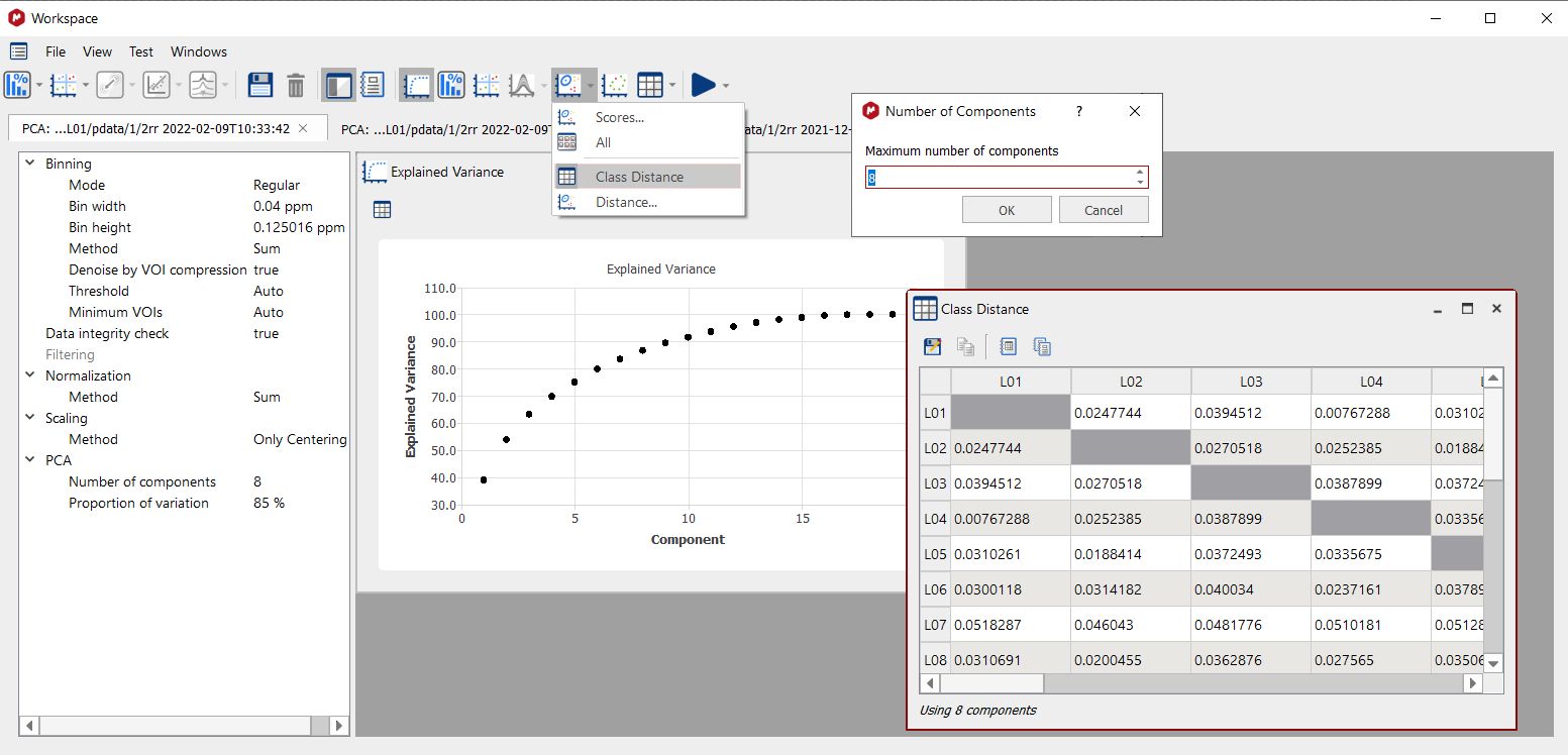
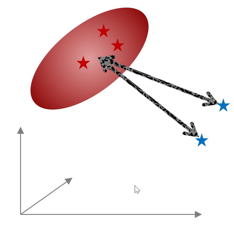
Distance Calculations

The Mahalanobis distance describes how many standard deviations a point is from the mean of a distribution. Distances are calculated between classes or between classes and an individual spectrum.

To compare classes, once you have defined several classes in one experiment, the less distance value will indicate that those classes will be ‘more similar’. Once you have selected the feature, a new dialog will be displayed to select the number of components to be used (maximum number is the total number of components, 8 in this case):

class_distance

Global Class distances are calculated from multi-dimensional ellipsoids using either the selected number of principal components or two selected PCs.

Global class

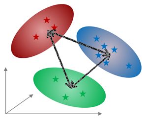
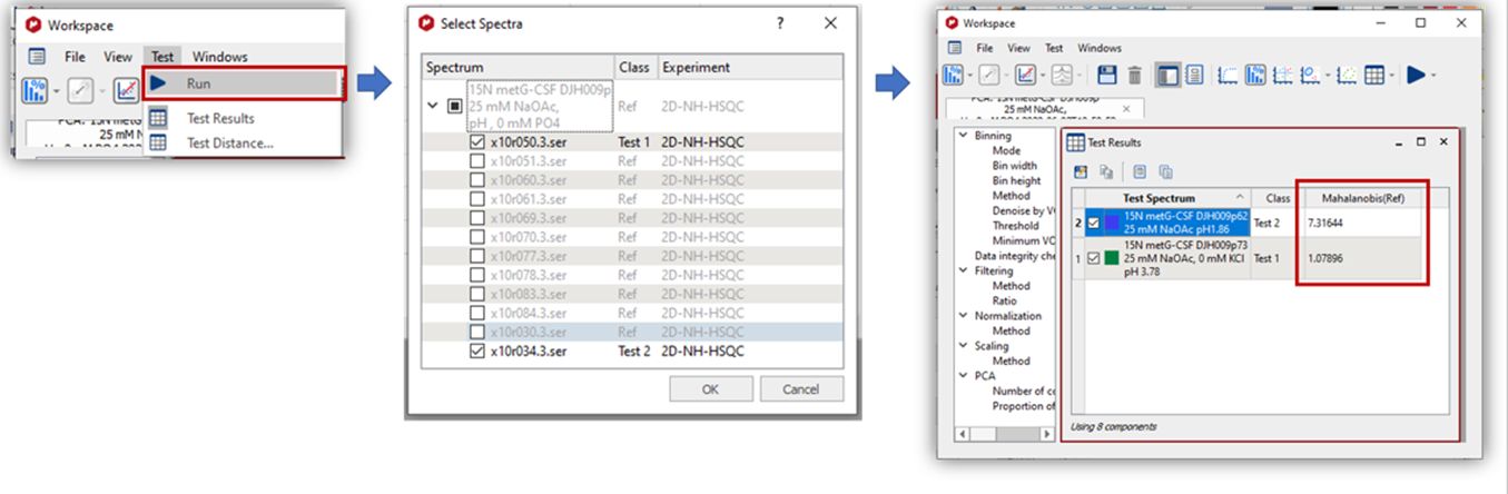
In the second case (to compare a test spectrum with different classes), once you have run the PCA and defined the classes, you could ‘test’ one (or several new spectra), the Mahalanobis distance against each of the classes (to get information about similar characteristics) .

test_distance_PCA

It is possible to measure the distance between classes and individual spectra. The spectra can be taken from any loaded document. It allows detecting to which class a spectrum belongs.

clases_PCA

This calculation is available via the Run command. Individual spectra can be selected.

run_pca

For the cases where each spectrum is in its own class, the distances are not Mahalanobis but Euclidean distances.

Further information can be found in this paper http://dx.doi.org/10.1208/s12249-017-0911-1